Range Trading StrategyOVERVIEW
The Range Trading Strategy is a systematic trading approach that identifies price ranges
from higher timeframe candles or trading sessions, tracks pivot points, and generates
trading signals when range extremes are mitigated and confirmed by pivot levels.
CORE CONCEPT
The strategy is based on the principle that when a candle (or session) closes within the
range of the previous candle (or session), that previous candle becomes a "range" with
identifiable high and low extremes. When price breaks through these extremes, it creates
trading opportunities that are confirmed by pivot levels.
RANGE DETECTION MODES
1. HTF (Higher Timeframe) Mode:
Automatically selects a higher timeframe based on the current chart timeframe
Uses request.security() to fetch HTF candle data
Range is created when an HTF candle closes within the previous HTF candle's range
The previous HTF candle's high and low become the range extremes
2. Sessions Mode:
- Divides the trading day into 4 sessions (UTC):
* Session 1: 00:00 - 06:00 (6 hours)
* Session 2: 06:00 - 12:00 (6 hours)
* Session 3: 12:00 - 20:00 (8 hours)
* Session 4: 20:00 - 00:00 (4 hours, spans midnight)
- Tracks high, low, and close for each session
- Range is created when a session closes within the previous session's range
- The previous session's high and low become the range extremes
PIVOT DETECTION
Pivots are detected based on candle color changes (bullish/bearish transitions):
1. Pivot Low:
Created when a bullish candle appears after a bearish candle
Pivot low = minimum of the current candle's low and previous candle's low
The pivot bar is the actual bar where the low was formed (current or previous bar)
2. Pivot High:
Created when a bearish candle appears after a bullish candle
Pivot high = maximum of the current candle's high and previous candle's high
The pivot bar is the actual bar where the high was formed (current or previous bar)
IMPORTANT: There is always only ONE active pivot high and ONE active pivot low at any
given time. When a new pivot is created, it replaces the previous one.
RANGE CREATION
A range is created when:
(HTF Mode) An HTF candle closes within the previous HTF candle's range AND a new HTF
candle has just started
(Sessions Mode) A session closes within the previous session's range AND a new session
has just started
Or Range Can Be Created when the Extreme of Another Range Gets Mitigated and We Have a Pivot low Just Above the Range Low or Pivot High just Below the Range High
Range Properties:
rangeHigh: The high extreme of the range
rangeLow: The low extreme of the range
highStartTime: The timestamp when the range high was actually formed (found by looping
backwards through bars)
lowStartTime: The timestamp when the range low was actually formed (found by looping
backwards through bars)
highMitigated / lowMitigated: Flags tracking whether each extreme has been broken
isSpecial: Flag indicating if this is a "special range" (see Special Ranges section)
RANGE MITIGATION
A range extreme is considered "mitigated" when price interacts with it:
High is mitigated when: high >= rangeHigh (any interaction at or above the level)
Low is mitigated when: low <= rangeLow (any interaction at or below the level)
Mitigation can happen:
At the moment of range creation (if price is already beyond the extreme)
At any point after range creation when price touches the extreme
SIGNAL GENERATION
1. Pending Signals:
When a range extreme is mitigated, a pending signal is created:
a) BEARISH Pending Signal:
- Triggered when: rangeHigh is mitigated
- Confirmation Level: Current pivotLow
- Signal is confirmed when: close < pivotLow
- Stop Loss: Current pivotHigh (at time of confirmation)
- Entry: Short position
Signal Confirmation
b) BULLISH Pending Signal:
- Triggered when: rangeLow is mitigated
- Confirmation Level: Current pivotHigh
- Signal is confirmed when: close > pivotHigh
- Stop Loss: Current pivotLow (at time of confirmation)
- Entry: Long position
IMPORTANT: There is only ever ONE pending bearish signal and ONE pending bullish signal
at any given time. When a new pending signal is created, it replaces the previous one
of the same type.
2. Signal Confirmation:
- Bearish: Confirmed when price closes below the pivot low (confirmation level)
- Bullish: Confirmed when price closes above the pivot high (confirmation level)
- Upon confirmation, a trade is entered immediately
- The confirmation line is drawn from the pivot bar to the confirmation bar
TRADE EXECUTION
When a signal is confirmed:
1. Position Management:
- Any existing position in the opposite direction is closed first
- Then the new position is entered
2. Stop Loss:
- Bearish (Short): Stop at pivotHigh
- Bullish (Long): Stop at pivotLow
3. Take Profit:
- Calculated using Risk:Reward Ratio (default 2:1)
- Risk = Distance from entry to stop loss
- Target = Entry ± (Risk × R:R Ratio)
- Can be disabled with "Stop Loss Only" toggle
4. Trade Comments:
- "Range Bear" for short trades
- "Range Bull" for long trades
SPECIAL RANGES
Special ranges are created when:
- A range high is mitigated AND the current pivotHigh is below the range high
- A range low is mitigated AND the current pivotLow is above the range low
In these cases:
- The pivot value is stored in an array (storedPivotHighs or storedPivotLows)
- A "special range" is created with only ONE extreme:
* If pivotHigh < rangeHigh: Creates a range with rangeHigh = pivotLow, rangeLow = na
* If pivotLow > rangeLow: Creates a range with rangeLow = pivotHigh, rangeHigh = na
- Special ranges can generate signals just like normal ranges
- If a special range is mitigated on the creation bar or the next bar, it is removed
entirely without generating signals (prevents false signals)
Special Ranges
REVERSE ON STOP LOSS
When enabled, if a stop loss is hit, the strategy automatically opens a trade in the
opposite direction:
1. Long Stop Loss Hit:
- Detects when: position_size > 0 AND position_size <= 0 AND low <= longStopLoss
- Action: Opens a SHORT position
- Stop Loss: Current pivotHigh
- Trade Comment: "Reverse on Stop"
2. Short Stop Loss Hit:
- Detects when: position_size < 0 AND position_size >= 0 AND high >= shortStopLoss
- Action: Opens a LONG position
- Stop Loss: Current pivotLow
- Trade Comment: "Reverse on Stop"
The reverse trade uses the same R:R ratio and respects the "Stop Loss Only" setting.
VISUAL ELEMENTS
1. Range Lines:
- Drawn from the time when the extreme was formed to the mitigation point (or current
time if not mitigated)
- High lines: Blue (or mitigated color if mitigated)
- Low lines: Red (or mitigated color if mitigated)
- Style: SOLID
- Width: 1
2. Confirmation Lines:
- Drawn when a signal is confirmed
- Extends from the pivot bar to the confirmation bar
- Bearish: Red, solid line
- Bullish: Green, solid line
- Width: 1
- Can be toggled on/off
STRATEGY SETTINGS
1. Range Detection Mode:
- HTF: Uses higher timeframe candles
- Sessions: Uses trading session boundaries
2. Auto HTF:
- Automatically selects HTF based on current chart timeframe
- Can be disabled to use manual HTF selection
3. Risk:Reward Ratio:
- Default: 2.0 (2:1)
- Minimum: 0.5
- Step: 0.5
4. Stop Loss Only:
- When enabled: Trades only have stop loss (no take profit)
- Trades close on stop loss or when opposite signal confirms
5. Reverse on Stop Loss:
- When enabled: Hitting a stop loss opens opposite trade with stop at opposing pivot
6. Max Ranges to Display:
- Limits the number of ranges kept in memory
- Oldest ranges are purged when limit is exceeded
KEY FEATURES
1. Dynamic Pivot Tracking:
- Pivots update on every candle color change
- Always maintains one high and one low pivot
2. Range Lifecycle:
- Ranges are created when price closes within previous range
- Ranges are tracked until mitigated
- Mitigation creates pending signals
- Signals are confirmed by pivot levels
3. Signal Priority:
- Only one pending signal of each type at a time
- New signals replace old ones
- Confirmation happens on close of bar
4. Position Management:
- Closes opposite positions before entering new trades
- Tracks stop loss levels for reverse functionality
- Respects pyramiding = 1 (only one position per direction)
5. Time-Based Drawing:
- Uses time coordinates instead of bar indices for line drawing
- Prevents "too far from current bar" errors
- Lines can extend to any historical point
USAGE NOTES
- Best suited for trending and ranging markets
- Works on any timeframe, but HTF mode adapts automatically
- Sessions mode is ideal for intraday trading
- Pivot detection requires clear candle color changes
- Range detection requires price to close within previous range
- Signals are generated on bar close, not intra-bar
The strategy combines range identification, pivot tracking, and signal confirmation to
create a systematic approach to trading breakouts and reversals based on price structure, past performance does not in any way predict future performance
ค้นหาในสคริปต์สำหรับ "high low"

Dynamic Equity Allocation Model"Cash is Trash"? Not Always. Here's Why Science Beats Guesswork.
Every retail trader knows the frustration: you draw support and resistance lines, you spot patterns, you follow market gurus on social media—and still, when the next bear market hits, your portfolio bleeds red. Meanwhile, institutional investors seem to navigate market turbulence with ease, preserving capital when markets crash and participating when they rally. What's their secret?
The answer isn't insider information or access to exotic derivatives. It's systematic, scientifically validated decision-making. While most retail traders rely on subjective chart analysis and emotional reactions, professional portfolio managers use quantitative models that remove emotion from the equation and process multiple streams of market information simultaneously.
This document presents exactly such a system—not a proprietary black box available only to hedge funds, but a fully transparent, academically grounded framework that any serious investor can understand and apply. The Dynamic Equity Allocation Model (DEAM) synthesizes decades of financial research from Nobel laureates and leading academics into a practical tool for tactical asset allocation.
Stop drawing colorful lines on your chart and start thinking like a quant. This isn't about predicting where the market goes next week—it's about systematically adjusting your risk exposure based on what the data actually tells you. When valuations scream danger, when volatility spikes, when credit markets freeze, when multiple warning signals align—that's when cash isn't trash. That's when cash saves your portfolio.
The irony of "cash is trash" rhetoric is that it ignores timing. Yes, being 100% cash for decades would be disastrous. But being 100% equities through every crisis is equally foolish. The sophisticated approach is dynamic: aggressive when conditions favor risk-taking, defensive when they don't. This model shows you how to make that decision systematically, not emotionally.
Whether you're managing your own retirement portfolio or seeking to understand how institutional allocation strategies work, this comprehensive analysis provides the theoretical foundation, mathematical implementation, and practical guidance to elevate your investment approach from amateur to professional.
The choice is yours: keep hoping your chart patterns work out, or start using the same quantitative methods that professionals rely on. The tools are here. The research is cited. The methodology is explained. All you need to do is read, understand, and apply.
The Dynamic Equity Allocation Model (DEAM) is a quantitative framework for systematic allocation between equities and cash, grounded in modern portfolio theory and empirical market research. The model integrates five scientifically validated dimensions of market analysis—market regime, risk metrics, valuation, sentiment, and macroeconomic conditions—to generate dynamic allocation recommendations ranging from 0% to 100% equity exposure. This work documents the theoretical foundations, mathematical implementation, and practical application of this multi-factor approach.
1. Introduction and Theoretical Background
1.1 The Limitations of Static Portfolio Allocation
Traditional portfolio theory, as formulated by Markowitz (1952) in his seminal work "Portfolio Selection," assumes an optimal static allocation where investors distribute their wealth across asset classes according to their risk aversion. This approach rests on the assumption that returns and risks remain constant over time. However, empirical research demonstrates that this assumption does not hold in reality. Fama and French (1989) showed that expected returns vary over time and correlate with macroeconomic variables such as the spread between long-term and short-term interest rates. Campbell and Shiller (1988) demonstrated that the price-earnings ratio possesses predictive power for future stock returns, providing a foundation for dynamic allocation strategies.
The academic literature on tactical asset allocation has evolved considerably over recent decades. Ilmanen (2011) argues in "Expected Returns" that investors can improve their risk-adjusted returns by considering valuation levels, business cycles, and market sentiment. The Dynamic Equity Allocation Model presented here builds on this research tradition and operationalizes these insights into a practically applicable allocation framework.
1.2 Multi-Factor Approaches in Asset Allocation
Modern financial research has shown that different factors capture distinct aspects of market dynamics and together provide a more robust picture of market conditions than individual indicators. Ross (1976) developed the Arbitrage Pricing Theory, a model that employs multiple factors to explain security returns. Following this multi-factor philosophy, DEAM integrates five complementary analytical dimensions, each tapping different information sources and collectively enabling comprehensive market understanding.
2. Data Foundation and Data Quality
2.1 Data Sources Used
The model draws its data exclusively from publicly available market data via the TradingView platform. This transparency and accessibility is a significant advantage over proprietary models that rely on non-public data. The data foundation encompasses several categories of market information, each capturing specific aspects of market dynamics.
First, price data for the S&P 500 Index is obtained through the SPDR S&P 500 ETF (ticker: SPY). The use of a highly liquid ETF instead of the index itself has practical reasons, as ETF data is available in real-time and reflects actual tradability. In addition to closing prices, high, low, and volume data are captured, which are required for calculating advanced volatility measures.
Fundamental corporate metrics are retrieved via TradingView's Financial Data API. These include earnings per share, price-to-earnings ratio, return on equity, debt-to-equity ratio, dividend yield, and share buyback yield. Cochrane (2011) emphasizes in "Presidential Address: Discount Rates" the central importance of valuation metrics for forecasting future returns, making these fundamental data a cornerstone of the model.
Volatility indicators are represented by the CBOE Volatility Index (VIX) and related metrics. The VIX, often referred to as the market's "fear gauge," measures the implied volatility of S&P 500 index options and serves as a proxy for market participants' risk perception. Whaley (2000) describes in "The Investor Fear Gauge" the construction and interpretation of the VIX and its use as a sentiment indicator.
Macroeconomic data includes yield curve information through US Treasury bonds of various maturities and credit risk premiums through the spread between high-yield bonds and risk-free government bonds. These variables capture the macroeconomic conditions and financing conditions relevant for equity valuation. Estrella and Hardouvelis (1991) showed that the shape of the yield curve has predictive power for future economic activity, justifying the inclusion of these data.
2.2 Handling Missing Data
A practical problem when working with financial data is dealing with missing or unavailable values. The model implements a fallback system where a plausible historical average value is stored for each fundamental metric. When current data is unavailable for a specific point in time, this fallback value is used. This approach ensures that the model remains functional even during temporary data outages and avoids systematic biases from missing data. The use of average values as fallback is conservative, as it generates neither overly optimistic nor pessimistic signals.
3. Component 1: Market Regime Detection
3.1 The Concept of Market Regimes
The idea that financial markets exist in different "regimes" or states that differ in their statistical properties has a long tradition in financial science. Hamilton (1989) developed regime-switching models that allow distinguishing between different market states with different return and volatility characteristics. The practical application of this theory consists of identifying the current market state and adjusting portfolio allocation accordingly.
DEAM classifies market regimes using a scoring system that considers three main dimensions: trend strength, volatility level, and drawdown depth. This multidimensional view is more robust than focusing on individual indicators, as it captures various facets of market dynamics. Classification occurs into six distinct regimes: Strong Bull, Bull Market, Neutral, Correction, Bear Market, and Crisis.
3.2 Trend Analysis Through Moving Averages
Moving averages are among the oldest and most widely used technical indicators and have also received attention in academic literature. Brock, Lakonishok, and LeBaron (1992) examined in "Simple Technical Trading Rules and the Stochastic Properties of Stock Returns" the profitability of trading rules based on moving averages and found evidence for their predictive power, although later studies questioned the robustness of these results when considering transaction costs.
The model calculates three moving averages with different time windows: a 20-day average (approximately one trading month), a 50-day average (approximately one quarter), and a 200-day average (approximately one trading year). The relationship of the current price to these averages and the relationship of the averages to each other provide information about trend strength and direction. When the price trades above all three averages and the short-term average is above the long-term, this indicates an established uptrend. The model assigns points based on these constellations, with longer-term trends weighted more heavily as they are considered more persistent.
3.3 Volatility Regimes
Volatility, understood as the standard deviation of returns, is a central concept of financial theory and serves as the primary risk measure. However, research has shown that volatility is not constant but changes over time and occurs in clusters—a phenomenon first documented by Mandelbrot (1963) and later formalized through ARCH and GARCH models (Engle, 1982; Bollerslev, 1986).
DEAM calculates volatility not only through the classic method of return standard deviation but also uses more advanced estimators such as the Parkinson estimator and the Garman-Klass estimator. These methods utilize intraday information (high and low prices) and are more efficient than simple close-to-close volatility estimators. The Parkinson estimator (Parkinson, 1980) uses the range between high and low of a trading day and is based on the recognition that this information reveals more about true volatility than just the closing price difference. The Garman-Klass estimator (Garman and Klass, 1980) extends this approach by additionally considering opening and closing prices.
The calculated volatility is annualized by multiplying it by the square root of 252 (the average number of trading days per year), enabling standardized comparability. The model compares current volatility with the VIX, the implied volatility from option prices. A low VIX (below 15) signals market comfort and increases the regime score, while a high VIX (above 35) indicates market stress and reduces the score. This interpretation follows the empirical observation that elevated volatility is typically associated with falling markets (Schwert, 1989).
3.4 Drawdown Analysis
A drawdown refers to the percentage decline from the highest point (peak) to the lowest point (trough) during a specific period. This metric is psychologically significant for investors as it represents the maximum loss experienced. Calmar (1991) developed the Calmar Ratio, which relates return to maximum drawdown, underscoring the practical relevance of this metric.
The model calculates current drawdown as the percentage distance from the highest price of the last 252 trading days (one year). A drawdown below 3% is considered negligible and maximally increases the regime score. As drawdown increases, the score decreases progressively, with drawdowns above 20% classified as severe and indicating a crisis or bear market regime. These thresholds are empirically motivated by historical market cycles, in which corrections typically encompassed 5-10% drawdowns, bear markets 20-30%, and crises over 30%.
3.5 Regime Classification
Final regime classification occurs through aggregation of scores from trend (40% weight), volatility (30%), and drawdown (30%). The higher weighting of trend reflects the empirical observation that trend-following strategies have historically delivered robust results (Moskowitz, Ooi, and Pedersen, 2012). A total score above 80 signals a strong bull market with established uptrend, low volatility, and minimal losses. At a score below 10, a crisis situation exists requiring defensive positioning. The six regime categories enable a differentiated allocation strategy that not only distinguishes binarily between bullish and bearish but allows gradual gradations.
4. Component 2: Risk-Based Allocation
4.1 Volatility Targeting as Risk Management Approach
The concept of volatility targeting is based on the idea that investors should maximize not returns but risk-adjusted returns. Sharpe (1966, 1994) defined with the Sharpe Ratio the fundamental concept of return per unit of risk, measured as volatility. Volatility targeting goes a step further and adjusts portfolio allocation to achieve constant target volatility. This means that in times of low market volatility, equity allocation is increased, and in times of high volatility, it is reduced.
Moreira and Muir (2017) showed in "Volatility-Managed Portfolios" that strategies that adjust their exposure based on volatility forecasts achieve higher Sharpe Ratios than passive buy-and-hold strategies. DEAM implements this principle by defining a target portfolio volatility (default 12% annualized) and adjusting equity allocation to achieve it. The mathematical foundation is simple: if market volatility is 20% and target volatility is 12%, equity allocation should be 60% (12/20 = 0.6), with the remaining 40% held in cash with zero volatility.
4.2 Market Volatility Calculation
Estimating current market volatility is central to the risk-based allocation approach. The model uses several volatility estimators in parallel and selects the higher value between traditional close-to-close volatility and the Parkinson estimator. This conservative choice ensures the model does not underestimate true volatility, which could lead to excessive risk exposure.
Traditional volatility calculation uses logarithmic returns, as these have mathematically advantageous properties (additive linkage over multiple periods). The logarithmic return is calculated as ln(P_t / P_{t-1}), where P_t is the price at time t. The standard deviation of these returns over a rolling 20-trading-day window is then multiplied by √252 to obtain annualized volatility. This annualization is based on the assumption of independently identically distributed returns, which is an idealization but widely accepted in practice.
The Parkinson estimator uses additional information from the trading range (High minus Low) of each day. The formula is: σ_P = (1/√(4ln2)) × √(1/n × Σln²(H_i/L_i)) × √252, where H_i and L_i are high and low prices. Under ideal conditions, this estimator is approximately five times more efficient than the close-to-close estimator (Parkinson, 1980), as it uses more information per observation.
4.3 Drawdown-Based Position Size Adjustment
In addition to volatility targeting, the model implements drawdown-based risk control. The logic is that deep market declines often signal further losses and therefore justify exposure reduction. This behavior corresponds with the concept of path-dependent risk tolerance: investors who have already suffered losses are typically less willing to take additional risk (Kahneman and Tversky, 1979).
The model defines a maximum portfolio drawdown as a target parameter (default 15%). Since portfolio volatility and portfolio drawdown are proportional to equity allocation (assuming cash has neither volatility nor drawdown), allocation-based control is possible. For example, if the market exhibits a 25% drawdown and target portfolio drawdown is 15%, equity allocation should be at most 60% (15/25).
4.4 Dynamic Risk Adjustment
An advanced feature of DEAM is dynamic adjustment of risk-based allocation through a feedback mechanism. The model continuously estimates what actual portfolio volatility and portfolio drawdown would result at the current allocation. If risk utilization (ratio of actual to target risk) exceeds 1.0, allocation is reduced by an adjustment factor that grows exponentially with overutilization. This implements a form of dynamic feedback that avoids overexposure.
Mathematically, a risk adjustment factor r_adjust is calculated: if risk utilization u > 1, then r_adjust = exp(-0.5 × (u - 1)). This exponential function ensures that moderate overutilization is gently corrected, while strong overutilization triggers drastic reductions. The factor 0.5 in the exponent was empirically calibrated to achieve a balanced ratio between sensitivity and stability.
5. Component 3: Valuation Analysis
5.1 Theoretical Foundations of Fundamental Valuation
DEAM's valuation component is based on the fundamental premise that the intrinsic value of a security is determined by its future cash flows and that deviations between market price and intrinsic value are eventually corrected. Graham and Dodd (1934) established in "Security Analysis" the basic principles of fundamental analysis that remain relevant today. Translated into modern portfolio context, this means that markets with high valuation metrics (high price-earnings ratios) should have lower expected returns than cheaply valued markets.
Campbell and Shiller (1988) developed the Cyclically Adjusted P/E Ratio (CAPE), which smooths earnings over a full business cycle. Their empirical analysis showed that this ratio has significant predictive power for 10-year returns. Asness, Moskowitz, and Pedersen (2013) demonstrated in "Value and Momentum Everywhere" that value effects exist not only in individual stocks but also in asset classes and markets.
5.2 Equity Risk Premium as Central Valuation Metric
The Equity Risk Premium (ERP) is defined as the expected excess return of stocks over risk-free government bonds. It is the theoretical heart of valuation analysis, as it represents the compensation investors demand for bearing equity risk. Damodaran (2012) discusses in "Equity Risk Premiums: Determinants, Estimation and Implications" various methods for ERP estimation.
DEAM calculates ERP not through a single method but combines four complementary approaches with different weights. This multi-method strategy increases estimation robustness and avoids dependence on single, potentially erroneous inputs.
The first method (35% weight) uses earnings yield, calculated as 1/P/E or directly from operating earnings data, and subtracts the 10-year Treasury yield. This method follows Fed Model logic (Yardeni, 2003), although this model has theoretical weaknesses as it does not consistently treat inflation (Asness, 2003).
The second method (30% weight) extends earnings yield by share buyback yield. Share buybacks are a form of capital return to shareholders and increase value per share. Boudoukh et al. (2007) showed in "The Total Shareholder Yield" that the sum of dividend yield and buyback yield is a better predictor of future returns than dividend yield alone.
The third method (20% weight) implements the Gordon Growth Model (Gordon, 1962), which models stock value as the sum of discounted future dividends. Under constant growth g assumption: Expected Return = Dividend Yield + g. The model estimates sustainable growth as g = ROE × (1 - Payout Ratio), where ROE is return on equity and payout ratio is the ratio of dividends to earnings. This formula follows from equity theory: unretained earnings are reinvested at ROE and generate additional earnings growth.
The fourth method (15% weight) combines total shareholder yield (Dividend + Buybacks) with implied growth derived from revenue growth. This method considers that companies with strong revenue growth should generate higher future earnings, even if current valuations do not yet fully reflect this.
The final ERP is the weighted average of these four methods. A high ERP (above 4%) signals attractive valuations and increases the valuation score to 95 out of 100 possible points. A negative ERP, where stocks have lower expected returns than bonds, results in a minimal score of 10.
5.3 Quality Adjustments to Valuation
Valuation metrics alone can be misleading if not interpreted in the context of company quality. A company with a low P/E may be cheap or fundamentally problematic. The model therefore implements quality adjustments based on growth, profitability, and capital structure.
Revenue growth above 10% annually adds 10 points to the valuation score, moderate growth above 5% adds 5 points. This adjustment reflects that growth has independent value (Modigliani and Miller, 1961, extended by later growth theory). Net margin above 15% signals pricing power and operational efficiency and increases the score by 5 points, while low margins below 8% indicate competitive pressure and subtract 5 points.
Return on equity (ROE) above 20% characterizes outstanding capital efficiency and increases the score by 5 points. Piotroski (2000) showed in "Value Investing: The Use of Historical Financial Statement Information" that fundamental quality signals such as high ROE can improve the performance of value strategies.
Capital structure is evaluated through the debt-to-equity ratio. A conservative ratio below 1.0 multiplies the valuation score by 1.2, while high leverage above 2.0 applies a multiplier of 0.8. This adjustment reflects that high debt constrains financial flexibility and can become problematic in crisis times (Korteweg, 2010).
6. Component 4: Sentiment Analysis
6.1 The Role of Sentiment in Financial Markets
Investor sentiment, defined as the collective psychological attitude of market participants, influences asset prices independently of fundamental data. Baker and Wurgler (2006, 2007) developed a sentiment index and showed that periods of high sentiment are followed by overvaluations that later correct. This insight justifies integrating a sentiment component into allocation decisions.
Sentiment is difficult to measure directly but can be proxied through market indicators. The VIX is the most widely used sentiment indicator, as it aggregates implied volatility from option prices. High VIX values reflect elevated uncertainty and risk aversion, while low values signal market comfort. Whaley (2009) refers to the VIX as the "Investor Fear Gauge" and documents its role as a contrarian indicator: extremely high values typically occur at market bottoms, while low values occur at tops.
6.2 VIX-Based Sentiment Assessment
DEAM uses statistical normalization of the VIX by calculating the Z-score: z = (VIX_current - VIX_average) / VIX_standard_deviation. The Z-score indicates how many standard deviations the current VIX is from the historical average. This approach is more robust than absolute thresholds, as it adapts to the average volatility level, which can vary over longer periods.
A Z-score below -1.5 (VIX is 1.5 standard deviations below average) signals exceptionally low risk perception and adds 40 points to the sentiment score. This may seem counterintuitive—shouldn't low fear be bullish? However, the logic follows the contrarian principle: when no one is afraid, everyone is already invested, and there is limited further upside potential (Zweig, 1973). Conversely, a Z-score above 1.5 (extreme fear) adds -40 points, reflecting market panic but simultaneously suggesting potential buying opportunities.
6.3 VIX Term Structure as Sentiment Signal
The VIX term structure provides additional sentiment information. Normally, the VIX trades in contango, meaning longer-term VIX futures have higher prices than short-term. This reflects that short-term volatility is currently known, while long-term volatility is more uncertain and carries a risk premium. The model compares the VIX with VIX9D (9-day volatility) and identifies backwardation (VIX > 1.05 × VIX9D) and steep backwardation (VIX > 1.15 × VIX9D).
Backwardation occurs when short-term implied volatility is higher than longer-term, which typically happens during market stress. Investors anticipate immediate turbulence but expect calming. Psychologically, this reflects acute fear. The model subtracts 15 points for backwardation and 30 for steep backwardation, as these constellations signal elevated risk. Simon and Wiggins (2001) analyzed the VIX futures curve and showed that backwardation is associated with market declines.
6.4 Safe-Haven Flows
During crisis times, investors flee from risky assets into safe havens: gold, US dollar, and Japanese yen. This "flight to quality" is a sentiment signal. The model calculates the performance of these assets relative to stocks over the last 20 trading days. When gold or the dollar strongly rise while stocks fall, this indicates elevated risk aversion.
The safe-haven component is calculated as the difference between safe-haven performance and stock performance. Positive values (safe havens outperform) subtract up to 20 points from the sentiment score, negative values (stocks outperform) add up to 10 points. The asymmetric treatment (larger deduction for risk-off than bonus for risk-on) reflects that risk-off movements are typically sharper and more informative than risk-on phases.
Baur and Lucey (2010) examined safe-haven properties of gold and showed that gold indeed exhibits negative correlation with stocks during extreme market movements, confirming its role as crisis protection.
7. Component 5: Macroeconomic Analysis
7.1 The Yield Curve as Economic Indicator
The yield curve, represented as yields of government bonds of various maturities, contains aggregated expectations about future interest rates, inflation, and economic growth. The slope of the yield curve has remarkable predictive power for recessions. Estrella and Mishkin (1998) showed that an inverted yield curve (short-term rates higher than long-term) predicts recessions with high reliability. This is because inverted curves reflect restrictive monetary policy: the central bank raises short-term rates to combat inflation, dampening economic activity.
DEAM calculates two spread measures: the 2-year-minus-10-year spread and the 3-month-minus-10-year spread. A steep, positive curve (spreads above 1.5% and 2% respectively) signals healthy growth expectations and generates the maximum yield curve score of 40 points. A flat curve (spreads near zero) reduces the score to 20 points. An inverted curve (negative spreads) is particularly alarming and results in only 10 points.
The choice of two different spreads increases analysis robustness. The 2-10 spread is most established in academic literature, while the 3M-10Y spread is often considered more sensitive, as the 3-month rate directly reflects current monetary policy (Ang, Piazzesi, and Wei, 2006).
7.2 Credit Conditions and Spreads
Credit spreads—the yield difference between risky corporate bonds and safe government bonds—reflect risk perception in the credit market. Gilchrist and Zakrajšek (2012) constructed an "Excess Bond Premium" that measures the component of credit spreads not explained by fundamentals and showed this is a predictor of future economic activity and stock returns.
The model approximates credit spread by comparing the yield of high-yield bond ETFs (HYG) with investment-grade bond ETFs (LQD). A narrow spread below 200 basis points signals healthy credit conditions and risk appetite, contributing 30 points to the macro score. Very wide spreads above 1000 basis points (as during the 2008 financial crisis) signal credit crunch and generate zero points.
Additionally, the model evaluates whether "flight to quality" is occurring, identified through strong performance of Treasury bonds (TLT) with simultaneous weakness in high-yield bonds. This constellation indicates elevated risk aversion and reduces the credit conditions score.
7.3 Financial Stability at Corporate Level
While the yield curve and credit spreads reflect macroeconomic conditions, financial stability evaluates the health of companies themselves. The model uses the aggregated debt-to-equity ratio and return on equity of the S&P 500 as proxies for corporate health.
A low leverage level below 0.5 combined with high ROE above 15% signals robust corporate balance sheets and generates 20 points. This combination is particularly valuable as it represents both defensive strength (low debt means crisis resistance) and offensive strength (high ROE means earnings power). High leverage above 1.5 generates only 5 points, as it implies vulnerability to interest rate increases and recessions.
Korteweg (2010) showed in "The Net Benefits to Leverage" that optimal debt maximizes firm value, but excessive debt increases distress costs. At the aggregated market level, high debt indicates fragilities that can become problematic during stress phases.
8. Component 6: Crisis Detection
8.1 The Need for Systematic Crisis Detection
Financial crises are rare but extremely impactful events that suspend normal statistical relationships. During normal market volatility, diversified portfolios and traditional risk management approaches function, but during systemic crises, seemingly independent assets suddenly correlate strongly, and losses exceed historical expectations (Longin and Solnik, 2001). This justifies a separate crisis detection mechanism that operates independently of regular allocation components.
Reinhart and Rogoff (2009) documented in "This Time Is Different: Eight Centuries of Financial Folly" recurring patterns in financial crises: extreme volatility, massive drawdowns, credit market dysfunction, and asset price collapse. DEAM operationalizes these patterns into quantifiable crisis indicators.
8.2 Multi-Signal Crisis Identification
The model uses a counter-based approach where various stress signals are identified and aggregated. This methodology is more robust than relying on a single indicator, as true crises typically occur simultaneously across multiple dimensions. A single signal may be a false alarm, but the simultaneous presence of multiple signals increases confidence.
The first indicator is a VIX above the crisis threshold (default 40), adding one point. A VIX above 60 (as in 2008 and March 2020) adds two additional points, as such extreme values are historically very rare. This tiered approach captures the intensity of volatility.
The second indicator is market drawdown. A drawdown above 15% adds one point, as corrections of this magnitude can be potential harbingers of larger crises. A drawdown above 25% adds another point, as historical bear markets typically encompass 25-40% drawdowns.
The third indicator is credit market spreads above 500 basis points, adding one point. Such wide spreads occur only during significant credit market disruptions, as in 2008 during the Lehman crisis.
The fourth indicator identifies simultaneous losses in stocks and bonds. Normally, Treasury bonds act as a hedge against equity risk (negative correlation), but when both fall simultaneously, this indicates systemic liquidity problems or inflation/stagflation fears. The model checks whether both SPY and TLT have fallen more than 10% and 5% respectively over 5 trading days, adding two points.
The fifth indicator is a volume spike combined with negative returns. Extreme trading volumes (above twice the 20-day average) with falling prices signal panic selling. This adds one point.
A crisis situation is diagnosed when at least 3 indicators trigger, a severe crisis at 5 or more indicators. These thresholds were calibrated through historical backtesting to identify true crises (2008, 2020) without generating excessive false alarms.
8.3 Crisis-Based Allocation Override
When a crisis is detected, the system overrides the normal allocation recommendation and caps equity allocation at maximum 25%. In a severe crisis, the cap is set at 10%. This drastic defensive posture follows the empirical observation that crises typically require time to develop and that early reduction can avoid substantial losses (Faber, 2007).
This override logic implements a "safety first" principle: in situations of existential danger to the portfolio, capital preservation becomes the top priority. Roy (1952) formalized this approach in "Safety First and the Holding of Assets," arguing that investors should primarily minimize ruin probability.
9. Integration and Final Allocation Calculation
9.1 Component Weighting
The final allocation recommendation emerges through weighted aggregation of the five components. The standard weighting is: Market Regime 35%, Risk Management 25%, Valuation 20%, Sentiment 15%, Macro 5%. These weights reflect both theoretical considerations and empirical backtesting results.
The highest weighting of market regime is based on evidence that trend-following and momentum strategies have delivered robust results across various asset classes and time periods (Moskowitz, Ooi, and Pedersen, 2012). Current market momentum is highly informative for the near future, although it provides no information about long-term expectations.
The substantial weighting of risk management (25%) follows from the central importance of risk control. Wealth preservation is the foundation of long-term wealth creation, and systematic risk management is demonstrably value-creating (Moreira and Muir, 2017).
The valuation component receives 20% weight, based on the long-term mean reversion of valuation metrics. While valuation has limited short-term predictive power (bull and bear markets can begin at any valuation), the long-term relationship between valuation and returns is robustly documented (Campbell and Shiller, 1988).
Sentiment (15%) and Macro (5%) receive lower weights, as these factors are subtler and harder to measure. Sentiment is valuable as a contrarian indicator at extremes but less informative in normal ranges. Macro variables such as the yield curve have strong predictive power for recessions, but the transmission from recessions to stock market performance is complex and temporally variable.
9.2 Model Type Adjustments
DEAM allows users to choose between four model types: Conservative, Balanced, Aggressive, and Adaptive. This choice modifies the final allocation through additive adjustments.
Conservative mode subtracts 10 percentage points from allocation, resulting in consistently more cautious positioning. This is suitable for risk-averse investors or those with limited investment horizons. Aggressive mode adds 10 percentage points, suitable for risk-tolerant investors with long horizons.
Adaptive mode implements procyclical adjustment based on short-term momentum: if the market has risen more than 5% in the last 20 days, 5 percentage points are added; if it has declined more than 5%, 5 points are subtracted. This logic follows the observation that short-term momentum persists (Jegadeesh and Titman, 1993), but the moderate size of adjustment avoids excessive timing bets.
Balanced mode makes no adjustment and uses raw model output. This neutral setting is suitable for investors who wish to trust model recommendations unchanged.
9.3 Smoothing and Stability
The allocation resulting from aggregation undergoes final smoothing through a simple moving average over 3 periods. This smoothing is crucial for model practicality, as it reduces frequent trading and thus transaction costs. Without smoothing, the model could fluctuate between adjacent allocations with every small input change.
The choice of 3 periods as smoothing window is a compromise between responsiveness and stability. Longer smoothing would excessively delay signals and impede response to true regime changes. Shorter or no smoothing would allow too much noise. Empirical tests showed that 3-period smoothing offers an optimal ratio between these goals.
10. Visualization and Interpretation
10.1 Main Output: Equity Allocation
DEAM's primary output is a time series from 0 to 100 representing the recommended percentage allocation to equities. This representation is intuitive: 100% means full investment in stocks (specifically: an S&P 500 ETF), 0% means complete cash position, and intermediate values correspond to mixed portfolios. A value of 60% means, for example: invest 60% of wealth in SPY, hold 40% in money market instruments or cash.
The time series is color-coded to enable quick visual interpretation. Green shades represent high allocations (above 80%, bullish), red shades low allocations (below 20%, bearish), and neutral colors middle allocations. The chart background is dynamically colored based on the signal, enhancing readability in different market phases.
10.2 Dashboard Metrics
A tabular dashboard presents key metrics compactly. This includes current allocation, cash allocation (complement), an aggregated signal (BULLISH/NEUTRAL/BEARISH), current market regime, VIX level, market drawdown, and crisis status.
Additionally, fundamental metrics are displayed: P/E Ratio, Equity Risk Premium, Return on Equity, Debt-to-Equity Ratio, and Total Shareholder Yield. This transparency allows users to understand model decisions and form their own assessments.
Component scores (Regime, Risk, Valuation, Sentiment, Macro) are also displayed, each normalized on a 0-100 scale. This shows which factors primarily drive the current recommendation. If, for example, the Risk score is very low (20) while other scores are moderate (50-60), this indicates that risk management considerations are pulling allocation down.
10.3 Component Breakdown (Optional)
Advanced users can display individual components as separate lines in the chart. This enables analysis of component dynamics: do all components move synchronously, or are there divergences? Divergences can be particularly informative. If, for example, the market regime is bullish (high score) but the valuation component is very negative, this signals an overbought market not fundamentally supported—a classic "bubble warning."
This feature is disabled by default to keep the chart clean but can be activated for deeper analysis.
10.4 Confidence Bands
The model optionally displays uncertainty bands around the main allocation line. These are calculated as ±1 standard deviation of allocation over a rolling 20-period window. Wide bands indicate high volatility of model recommendations, suggesting uncertain market conditions. Narrow bands indicate stable recommendations.
This visualization implements a concept of epistemic uncertainty—uncertainty about the model estimate itself, not just market volatility. In phases where various indicators send conflicting signals, the allocation recommendation becomes more volatile, manifesting in wider bands. Users can understand this as a warning to act more cautiously or consult alternative information sources.
11. Alert System
11.1 Allocation Alerts
DEAM implements an alert system that notifies users of significant events. Allocation alerts trigger when smoothed allocation crosses certain thresholds. An alert is generated when allocation reaches 80% (from below), signaling strong bullish conditions. Another alert triggers when allocation falls to 20%, indicating defensive positioning.
These thresholds are not arbitrary but correspond with boundaries between model regimes. An allocation of 80% roughly corresponds to a clear bull market regime, while 20% corresponds to a bear market regime. Alerts at these points are therefore informative about fundamental regime shifts.
11.2 Crisis Alerts
Separate alerts trigger upon detection of crisis and severe crisis. These alerts have highest priority as they signal large risks. A crisis alert should prompt investors to review their portfolio and potentially take defensive measures beyond the automatic model recommendation (e.g., hedging through put options, rebalancing to more defensive sectors).
11.3 Regime Change Alerts
An alert triggers upon change of market regime (e.g., from Neutral to Correction, or from Bull Market to Strong Bull). Regime changes are highly informative events that typically entail substantial allocation changes. These alerts enable investors to proactively respond to changes in market dynamics.
11.4 Risk Breach Alerts
A specialized alert triggers when actual portfolio risk utilization exceeds target parameters by 20%. This is a warning signal that the risk management system is reaching its limits, possibly because market volatility is rising faster than allocation can be reduced. In such situations, investors should consider manual interventions.
12. Practical Application and Limitations
12.1 Portfolio Implementation
DEAM generates a recommendation for allocation between equities (S&P 500) and cash. Implementation by an investor can take various forms. The most direct method is using an S&P 500 ETF (e.g., SPY, VOO) for equity allocation and a money market fund or savings account for cash allocation.
A rebalancing strategy is required to synchronize actual allocation with model recommendation. Two approaches are possible: (1) rule-based rebalancing at every 10% deviation between actual and target, or (2) time-based monthly rebalancing. Both have trade-offs between responsiveness and transaction costs. Empirical evidence (Jaconetti, Kinniry, and Zilbering, 2010) suggests rebalancing frequency has moderate impact on performance, and investors should optimize based on their transaction costs.
12.2 Adaptation to Individual Preferences
The model offers numerous adjustment parameters. Component weights can be modified if investors place more or less belief in certain factors. A fundamentally-oriented investor might increase valuation weight, while a technical trader might increase regime weight.
Risk target parameters (target volatility, max drawdown) should be adapted to individual risk tolerance. Younger investors with long investment horizons can choose higher target volatility (15-18%), while retirees may prefer lower volatility (8-10%). This adjustment systematically shifts average equity allocation.
Crisis thresholds can be adjusted based on preference for sensitivity versus specificity of crisis detection. Lower thresholds (e.g., VIX > 35 instead of 40) increase sensitivity (more crises are detected) but reduce specificity (more false alarms). Higher thresholds have the reverse effect.
12.3 Limitations and Disclaimers
DEAM is based on historical relationships between indicators and market performance. There is no guarantee these relationships will persist in the future. Structural changes in markets (e.g., through regulation, technology, or central bank policy) can break established patterns. This is the fundamental problem of induction in financial science (Taleb, 2007).
The model is optimized for US equities (S&P 500). Application to other markets (international stocks, bonds, commodities) would require recalibration. The indicators and thresholds are specific to the statistical properties of the US equity market.
The model cannot eliminate losses. Even with perfect crisis prediction, an investor following the model would lose money in bear markets—just less than a buy-and-hold investor. The goal is risk-adjusted performance improvement, not risk elimination.
Transaction costs are not modeled. In practice, spreads, commissions, and taxes reduce net returns. Frequent trading can cause substantial costs. Model smoothing helps minimize this, but users should consider their specific cost situation.
The model reacts to information; it does not anticipate it. During sudden shocks (e.g., 9/11, COVID-19 lockdowns), the model can only react after price movements, not before. This limitation is inherent to all reactive systems.
12.4 Relationship to Other Strategies
DEAM is a tactical asset allocation approach and should be viewed as a complement, not replacement, for strategic asset allocation. Brinson, Hood, and Beebower (1986) showed in their influential study "Determinants of Portfolio Performance" that strategic asset allocation (long-term policy allocation) explains the majority of portfolio performance, but this leaves room for tactical adjustments based on market timing.
The model can be combined with value and momentum strategies at the individual stock level. While DEAM controls overall market exposure, within-equity decisions can be optimized through stock-picking models. This separation between strategic (market exposure) and tactical (stock selection) levels follows classical portfolio theory.
The model does not replace diversification across asset classes. A complete portfolio should also include bonds, international stocks, real estate, and alternative investments. DEAM addresses only the US equity allocation decision within a broader portfolio.
13. Scientific Foundation and Evaluation
13.1 Theoretical Consistency
DEAM's components are based on established financial theory and empirical evidence. The market regime component follows from regime-switching models (Hamilton, 1989) and trend-following literature. The risk management component implements volatility targeting (Moreira and Muir, 2017) and modern portfolio theory (Markowitz, 1952). The valuation component is based on discounted cash flow theory and empirical value research (Campbell and Shiller, 1988; Fama and French, 1992). The sentiment component integrates behavioral finance (Baker and Wurgler, 2006). The macro component uses established business cycle indicators (Estrella and Mishkin, 1998).
This theoretical grounding distinguishes DEAM from purely data-mining-based approaches that identify patterns without causal theory. Theory-guided models have greater probability of functioning out-of-sample, as they are based on fundamental mechanisms, not random correlations (Lo and MacKinlay, 1990).
13.2 Empirical Validation
While this document does not present detailed backtest analysis, it should be noted that rigorous validation of a tactical asset allocation model should include several elements:
In-sample testing establishes whether the model functions at all in the data on which it was calibrated. Out-of-sample testing is crucial: the model should be tested in time periods not used for development. Walk-forward analysis, where the model is successively trained on rolling windows and tested in the next window, approximates real implementation.
Performance metrics should be risk-adjusted. Pure return consideration is misleading, as higher returns often only compensate for higher risk. Sharpe Ratio, Sortino Ratio, Calmar Ratio, and Maximum Drawdown are relevant metrics. Comparison with benchmarks (Buy-and-Hold S&P 500, 60/40 Stock/Bond portfolio) contextualizes performance.
Robustness checks test sensitivity to parameter variation. If the model only functions at specific parameter settings, this indicates overfitting. Robust models show consistent performance over a range of plausible parameters.
13.3 Comparison with Existing Literature
DEAM fits into the broader literature on tactical asset allocation. Faber (2007) presented a simple momentum-based timing system that goes long when the market is above its 10-month average, otherwise cash. This simple system avoided large drawdowns in bear markets. DEAM can be understood as a sophistication of this approach that integrates multiple information sources.
Ilmanen (2011) discusses various timing factors in "Expected Returns" and argues for multi-factor approaches. DEAM operationalizes this philosophy. Asness, Moskowitz, and Pedersen (2013) showed that value and momentum effects work across asset classes, justifying cross-asset application of regime and valuation signals.
Ang (2014) emphasizes in "Asset Management: A Systematic Approach to Factor Investing" the importance of systematic, rule-based approaches over discretionary decisions. DEAM is fully systematic and eliminates emotional biases that plague individual investors (overconfidence, hindsight bias, loss aversion).
References
Ang, A. (2014) *Asset Management: A Systematic Approach to Factor Investing*. Oxford: Oxford University Press.
Ang, A., Piazzesi, M. and Wei, M. (2006) 'What does the yield curve tell us about GDP growth?', *Journal of Econometrics*, 131(1-2), pp. 359-403.
Asness, C.S. (2003) 'Fight the Fed Model', *The Journal of Portfolio Management*, 30(1), pp. 11-24.
Asness, C.S., Moskowitz, T.J. and Pedersen, L.H. (2013) 'Value and Momentum Everywhere', *The Journal of Finance*, 68(3), pp. 929-985.
Baker, M. and Wurgler, J. (2006) 'Investor Sentiment and the Cross-Section of Stock Returns', *The Journal of Finance*, 61(4), pp. 1645-1680.
Baker, M. and Wurgler, J. (2007) 'Investor Sentiment in the Stock Market', *Journal of Economic Perspectives*, 21(2), pp. 129-152.
Baur, D.G. and Lucey, B.M. (2010) 'Is Gold a Hedge or a Safe Haven? An Analysis of Stocks, Bonds and Gold', *Financial Review*, 45(2), pp. 217-229.
Bollerslev, T. (1986) 'Generalized Autoregressive Conditional Heteroskedasticity', *Journal of Econometrics*, 31(3), pp. 307-327.
Boudoukh, J., Michaely, R., Richardson, M. and Roberts, M.R. (2007) 'On the Importance of Measuring Payout Yield: Implications for Empirical Asset Pricing', *The Journal of Finance*, 62(2), pp. 877-915.
Brinson, G.P., Hood, L.R. and Beebower, G.L. (1986) 'Determinants of Portfolio Performance', *Financial Analysts Journal*, 42(4), pp. 39-44.
Brock, W., Lakonishok, J. and LeBaron, B. (1992) 'Simple Technical Trading Rules and the Stochastic Properties of Stock Returns', *The Journal of Finance*, 47(5), pp. 1731-1764.
Calmar, T.W. (1991) 'The Calmar Ratio', *Futures*, October issue.
Campbell, J.Y. and Shiller, R.J. (1988) 'The Dividend-Price Ratio and Expectations of Future Dividends and Discount Factors', *Review of Financial Studies*, 1(3), pp. 195-228.
Cochrane, J.H. (2011) 'Presidential Address: Discount Rates', *The Journal of Finance*, 66(4), pp. 1047-1108.
Damodaran, A. (2012) *Equity Risk Premiums: Determinants, Estimation and Implications*. Working Paper, Stern School of Business.
Engle, R.F. (1982) 'Autoregressive Conditional Heteroskedasticity with Estimates of the Variance of United Kingdom Inflation', *Econometrica*, 50(4), pp. 987-1007.
Estrella, A. and Hardouvelis, G.A. (1991) 'The Term Structure as a Predictor of Real Economic Activity', *The Journal of Finance*, 46(2), pp. 555-576.
Estrella, A. and Mishkin, F.S. (1998) 'Predicting U.S. Recessions: Financial Variables as Leading Indicators', *Review of Economics and Statistics*, 80(1), pp. 45-61.
Faber, M.T. (2007) 'A Quantitative Approach to Tactical Asset Allocation', *The Journal of Wealth Management*, 9(4), pp. 69-79.
Fama, E.F. and French, K.R. (1989) 'Business Conditions and Expected Returns on Stocks and Bonds', *Journal of Financial Economics*, 25(1), pp. 23-49.
Fama, E.F. and French, K.R. (1992) 'The Cross-Section of Expected Stock Returns', *The Journal of Finance*, 47(2), pp. 427-465.
Garman, M.B. and Klass, M.J. (1980) 'On the Estimation of Security Price Volatilities from Historical Data', *Journal of Business*, 53(1), pp. 67-78.
Gilchrist, S. and Zakrajšek, E. (2012) 'Credit Spreads and Business Cycle Fluctuations', *American Economic Review*, 102(4), pp. 1692-1720.
Gordon, M.J. (1962) *The Investment, Financing, and Valuation of the Corporation*. Homewood: Irwin.
Graham, B. and Dodd, D.L. (1934) *Security Analysis*. New York: McGraw-Hill.
Hamilton, J.D. (1989) 'A New Approach to the Economic Analysis of Nonstationary Time Series and the Business Cycle', *Econometrica*, 57(2), pp. 357-384.
Ilmanen, A. (2011) *Expected Returns: An Investor's Guide to Harvesting Market Rewards*. Chichester: Wiley.
Jaconetti, C.M., Kinniry, F.M. and Zilbering, Y. (2010) 'Best Practices for Portfolio Rebalancing', *Vanguard Research Paper*.
Jegadeesh, N. and Titman, S. (1993) 'Returns to Buying Winners and Selling Losers: Implications for Stock Market Efficiency', *The Journal of Finance*, 48(1), pp. 65-91.
Kahneman, D. and Tversky, A. (1979) 'Prospect Theory: An Analysis of Decision under Risk', *Econometrica*, 47(2), pp. 263-292.
Korteweg, A. (2010) 'The Net Benefits to Leverage', *The Journal of Finance*, 65(6), pp. 2137-2170.
Lo, A.W. and MacKinlay, A.C. (1990) 'Data-Snooping Biases in Tests of Financial Asset Pricing Models', *Review of Financial Studies*, 3(3), pp. 431-467.
Longin, F. and Solnik, B. (2001) 'Extreme Correlation of International Equity Markets', *The Journal of Finance*, 56(2), pp. 649-676.
Mandelbrot, B. (1963) 'The Variation of Certain Speculative Prices', *The Journal of Business*, 36(4), pp. 394-419.
Markowitz, H. (1952) 'Portfolio Selection', *The Journal of Finance*, 7(1), pp. 77-91.
Modigliani, F. and Miller, M.H. (1961) 'Dividend Policy, Growth, and the Valuation of Shares', *The Journal of Business*, 34(4), pp. 411-433.
Moreira, A. and Muir, T. (2017) 'Volatility-Managed Portfolios', *The Journal of Finance*, 72(4), pp. 1611-1644.
Moskowitz, T.J., Ooi, Y.H. and Pedersen, L.H. (2012) 'Time Series Momentum', *Journal of Financial Economics*, 104(2), pp. 228-250.
Parkinson, M. (1980) 'The Extreme Value Method for Estimating the Variance of the Rate of Return', *Journal of Business*, 53(1), pp. 61-65.
Piotroski, J.D. (2000) 'Value Investing: The Use of Historical Financial Statement Information to Separate Winners from Losers', *Journal of Accounting Research*, 38, pp. 1-41.
Reinhart, C.M. and Rogoff, K.S. (2009) *This Time Is Different: Eight Centuries of Financial Folly*. Princeton: Princeton University Press.
Ross, S.A. (1976) 'The Arbitrage Theory of Capital Asset Pricing', *Journal of Economic Theory*, 13(3), pp. 341-360.
Roy, A.D. (1952) 'Safety First and the Holding of Assets', *Econometrica*, 20(3), pp. 431-449.
Schwert, G.W. (1989) 'Why Does Stock Market Volatility Change Over Time?', *The Journal of Finance*, 44(5), pp. 1115-1153.
Sharpe, W.F. (1966) 'Mutual Fund Performance', *The Journal of Business*, 39(1), pp. 119-138.
Sharpe, W.F. (1994) 'The Sharpe Ratio', *The Journal of Portfolio Management*, 21(1), pp. 49-58.
Simon, D.P. and Wiggins, R.A. (2001) 'S&P Futures Returns and Contrary Sentiment Indicators', *Journal of Futures Markets*, 21(5), pp. 447-462.
Taleb, N.N. (2007) *The Black Swan: The Impact of the Highly Improbable*. New York: Random House.
Whaley, R.E. (2000) 'The Investor Fear Gauge', *The Journal of Portfolio Management*, 26(3), pp. 12-17.
Whaley, R.E. (2009) 'Understanding the VIX', *The Journal of Portfolio Management*, 35(3), pp. 98-105.
Yardeni, E. (2003) 'Stock Valuation Models', *Topical Study*, 51, Yardeni Research.
Zweig, M.E. (1973) 'An Investor Expectations Stock Price Predictive Model Using Closed-End Fund Premiums', *The Journal of Finance*, 28(1), pp. 67-78.

SMC Structures and FVGสวัสดีครับ! ผมจะอธิบายอินดิเคเตอร์ "SMC Structures and FVG + MACD" ที่คุณให้มาอย่างละเอียดในแต่ละส่วน เพื่อให้คุณเข้าใจการทำงานของมันอย่างถ่องแท้ครับ
อินดิเคเตอร์นี้เป็นการผสมผสานแนวคิดของ Smart Money Concept (SMC) ซึ่งเน้นการวิเคราะห์โครงสร้างตลาด (Market Structure) และ Fair Value Gap (FVG) เข้ากับอินดิเคเตอร์ MACD เพื่อใช้เป็นตัวกรองหรือตัวยืนยันสัญญาณ Choch/BoS (Change of Character / Break of Structure)
1. ภาพรวมอินดิเคเตอร์ (Overall Purpose)
อินดิเคเตอร์นี้มีจุดประสงค์หลักคือ:
ระบุโครงสร้างตลาด: ตีเส้นและป้ายกำกับ Choch (Change of Character) และ BoS (Break of Structure) บนกราฟโดยอัตโนมัติ
ผสานการยืนยันด้วย MACD: สัญญาณ Choch/BoS จะถูกพิจารณาก็ต่อเมื่อ MACD Histogram เกิดการตัดขึ้นหรือลง (Zero Cross) ในทิศทางที่สอดคล้องกัน
แสดง Fair Value Gap (FVG): หากเปิดใช้งาน จะมีการตีกล่อง FVG บนกราฟ
แสดงระดับ Fibonacci: คำนวณและแสดงระดับ Fibonacci ที่สำคัญตามโครงสร้างตลาดปัจจุบัน
ปรับตาม Timeframe: การคำนวณและการแสดงผลทั้งหมดจะปรับตาม Timeframe ที่คุณกำลังใช้งานอยู่โดยอัตโนมัติ
2. ส่วนประกอบหลักของโค้ด (Code Breakdown)
โค้ดนี้สามารถแบ่งออกเป็นส่วนหลัก ๆ ได้ดังนี้:
2.1 Inputs (การตั้งค่า)
ส่วนนี้คือตัวแปรที่คุณสามารถปรับแต่งได้ในหน้าต่างการตั้งค่าของอินดิเคเตอร์ (คลิกที่รูปฟันเฟืองข้างชื่ออินดิเคเตอร์บนกราฟ)
MACD Settings (ตั้งค่า MACD):
fast_len: ความยาวของ Fast EMA สำหรับ MACD (ค่าเริ่มต้น 12)
slow_len: ความยาวของ Slow EMA สำหรับ MACD (ค่าเริ่มต้น 26)
signal_len: ความยาวของ Signal Line สำหรับ MACD (ค่าเริ่มต้น 9)
= ta.macd(close, fast_len, slow_len, signal_len): คำนวณค่า MACD Line, Signal Line และ Histogram โดยใช้ราคาปิด (close) และค่าความยาวที่กำหนด
is_bullish_macd_cross: ตรวจสอบว่า MACD Histogram ตัดขึ้นเหนือเส้น 0 (จากค่าลบเป็นบวก)
is_bearish_macd_cross: ตรวจสอบว่า MACD Histogram ตัดลงใต้เส้น 0 (จากค่าบวกเป็นลบ)
Fear Value Gap (FVG) Settings:
isFvgToShow: (Boolean) เปิด/ปิดการแสดง FVG บนกราฟ
bullishFvgColor: สีสำหรับ Bullish FVG
bearishFvgColor: สีสำหรับ Bearish FVG
mitigatedFvgColor: สีสำหรับ FVG ที่ถูก Mitigate (ลดทอน) แล้ว
fvgHistoryNbr: จำนวน FVG ย้อนหลังที่จะแสดง
isMitigatedFvgToReduce: (Boolean) เปิด/ปิดการลดขนาด FVG เมื่อถูก Mitigate
Structures (โครงสร้างตลาด) Settings:
isStructBodyCandleBreak: (Boolean) หากเป็น true การ Break จะต้องเกิดขึ้นด้วย เนื้อเทียน ที่ปิดเหนือ/ใต้ Swing High/Low หากเป็น false แค่ไส้เทียนทะลุก็ถือว่า Break
isCurrentStructToShow: (Boolean) เปิด/ปิดการแสดงเส้นโครงสร้างตลาดปัจจุบัน (เส้นสีน้ำเงินในภาพตัวอย่าง)
pivot_len: ความยาวของแท่งเทียนที่ใช้ในการมองหาจุด Pivot (Swing High/Low) ยิ่งค่าน้อยยิ่งจับ Swing เล็กๆ ได้, ยิ่งค่ามากยิ่งจับ Swing ใหญ่ๆ ได้
bullishBosColor, bearishBosColor: สีสำหรับเส้นและป้าย BOS ขาขึ้น/ขาลง
bosLineStyleOption, bosLineWidth: สไตล์ (Solid, Dotted, Dashed) และความหนาของเส้น BOS
bullishChochColor, bearishChochColor: สีสำหรับเส้นและป้าย CHoCH ขาขึ้น/ขาลง
chochLineStyleOption, chochLineWidth: สไตล์ (Solid, Dotted, Dashed) และความหนาของเส้น CHoCH
currentStructColor, currentStructLineStyleOption, currentStructLineWidth: สี, สไตล์ และความหนาของเส้นโครงสร้างตลาดปัจจุบัน
structHistoryNbr: จำนวนการ Break (Choch/BoS) ย้อนหลังที่จะแสดง
Structure Fibonacci (จากโค้ดต้นฉบับ):
เป็นชุด Input สำหรับเปิด/ปิด, กำหนดค่า, สี, สไตล์ และความหนาของเส้น Fibonacci Levels ต่างๆ (0.786, 0.705, 0.618, 0.5, 0.382) ที่จะถูกคำนวณจากโครงสร้างตลาดปัจจุบัน
2.2 Helper Functions (ฟังก์ชันช่วยทำงาน)
getLineStyle(lineOption): ฟังก์ชันนี้ใช้แปลงค่า String ที่เลือกจาก Input (เช่น "─", "┈", "╌") ให้เป็นรูปแบบ line.style_ ที่ Pine Script เข้าใจ
get_structure_highest_bar(lookback): ฟังก์ชันนี้พยายามหา Bar Index ของแท่งเทียนที่ทำ Swing High ภายในช่วง lookback ที่กำหนด
get_structure_lowest_bar(lookback): ฟังก์ชันนี้พยายามหา Bar Index ของแท่งเทียนที่ทำ Swing Low ภายในช่วง lookback ที่กำหนด
is_structure_high_broken(...): ฟังก์ชันนี้ตรวจสอบว่าราคาปัจจุบันได้ Break เหนือ _structureHigh (Swing High) หรือไม่ โดยพิจารณาจาก _highStructBreakPrice (ราคาปิดหรือราคา High ขึ้นอยู่กับการตั้งค่า isStructBodyCandleBreak)
FVGDraw(...): ฟังก์ชันนี้รับ Arrays ของ FVG Boxes, Types, Mitigation Status และ Labels มาประมวลผล เพื่ออัปเดตสถานะของ FVG (เช่น ถูก Mitigate หรือไม่) และปรับขนาด/ตำแหน่งของ FVG Box และ Label บนกราฟ
2.3 Global Variables (ตัวแปรทั่วทั้งอินดิเคเตอร์)
เป็นตัวแปรที่ประกาศด้วย var ซึ่งหมายความว่าค่าของมันจะถูกเก็บไว้และอัปเดตในแต่ละแท่งเทียน (persists across bars)
structureLines, structureLabels: Arrays สำหรับเก็บอ็อบเจกต์ line และ label ของเส้น Choch/BoS ที่วาดบนกราฟ
fvgBoxes, fvgTypes, fvgLabels, isFvgMitigated: Arrays สำหรับเก็บข้อมูลของ FVG Boxes และสถานะต่างๆ
structureHigh, structureLow: เก็บราคาของ Swing High/Low ที่สำคัญของโครงสร้างตลาดปัจจุบัน
structureHighStartIndex, structureLowStartIndex: เก็บ Bar Index ของจุดเริ่มต้นของ Swing High/Low ที่สำคัญ
structureDirection: เก็บสถานะของทิศทางโครงสร้างตลาด (1 = Bullish, 2 = Bearish, 0 = Undefined)
fiboXPrice, fiboXStartIndex, fiboXLine, fiboXLabel: ตัวแปรสำหรับเก็บข้อมูลและอ็อบเจกต์ของเส้น Fibonacci Levels
isBOSAlert, isCHOCHAlert: (Boolean) ใช้สำหรับส่งสัญญาณ Alert (หากมีการตั้งค่า Alert ไว้)
2.4 FVG Processing (การประมวลผล FVG)
ส่วนนี้จะตรวจสอบเงื่อนไขการเกิด FVG (Bullish FVG: high < low , Bearish FVG: low > high )
หากเกิด FVG และ isFvgToShow เป็น true จะมีการสร้าง box และ label ใหม่เพื่อแสดง FVG บนกราฟ
มีการจัดการ fvgBoxes และ fvgLabels เพื่อจำกัดจำนวน FVG ที่แสดงตาม fvgHistoryNbr และลบ FVG เก่าออก
ฟังก์ชัน FVGDraw จะถูกเรียกเพื่ออัปเดตสถานะของ FVG (เช่น การถูก Mitigate) และปรับการแสดงผล
2.5 Structures Processing (การประมวลผลโครงสร้างตลาด)
Initialization: ที่ bar_index == 0 (แท่งเทียนแรกของกราฟ) จะมีการกำหนดค่าเริ่มต้นให้กับ structureHigh, structureLow, structureHighStartIndex, structureLowStartIndex
Finding Current High/Low: highest, highestBar, lowest, lowestBar ถูกใช้เพื่อหา High/Low ที่สุดและ Bar Index ของมันใน 10 แท่งล่าสุด (หรือทั้งหมดหากกราฟสั้นกว่า 10 แท่ง)
Calculating Structure Max/Min Bar: structureMaxBar และ structureMinBar ใช้ฟังก์ชัน get_structure_highest_bar และ get_structure_lowest_bar เพื่อหา Bar Index ของ Swing High/Low ที่แท้จริง (ไม่ใช่แค่ High/Low ที่สุดใน lookback แต่เป็นจุด Pivot ที่สมบูรณ์)
Break Price: lowStructBreakPrice และ highStructBreakPrice จะเป็นราคาปิด (close) หรือราคา Low/High ขึ้นอยู่กับ isStructBodyCandleBreak
isStuctureLowBroken / isStructureHighBroken: เงื่อนไขเหล่านี้ตรวจสอบว่าราคาได้ทำลาย structureLow หรือ structureHigh หรือไม่ โดยพิจารณาจากราคา Break, ราคาแท่งก่อนหน้า และ Bar Index ของจุดเริ่มต้นโครงสร้าง
Choch/BoS Logic (ส่วนสำคัญที่ถูกผสานกับ MACD):
if(isStuctureLowBroken and is_bearish_macd_cross): นี่คือจุดที่ MACD เข้ามามีบทบาท หากราคาทำลาย structureLow (สัญญาณขาลง) และ MACD Histogram เกิด Bearish Zero Cross (is_bearish_macd_cross เป็น true) อินดิเคเตอร์จะพิจารณาว่าเป็น Choch หรือ BoS
หาก structureDirection == 1 (เดิมเป็นขาขึ้น) หรือ 0 (ยังไม่กำหนด) จะตีเป็น "CHoCH" (เปลี่ยนทิศทางโครงสร้างเป็นขาลง)
หาก structureDirection == 2 (เดิมเป็นขาลง) จะตีเป็น "BOS" (ยืนยันโครงสร้างขาลง)
มีการสร้าง line.new และ label.new เพื่อวาดเส้นและป้ายกำกับ
structureDirection จะถูกอัปเดตเป็น 1 (Bullish)
structureHighStartIndex, structureLowStartIndex, structureHigh, structureLow จะถูกอัปเดตเพื่อกำหนดโครงสร้างใหม่
else if(isStructureHighBroken and is_bullish_macd_cross): เช่นกันสำหรับขาขึ้น หากราคาทำลาย structureHigh (สัญญาณขาขึ้น) และ MACD Histogram เกิด Bullish Zero Cross (is_bullish_macd_cross เป็น true) อินดิเคเตอร์จะพิจารณาว่าเป็น Choch หรือ BoS
หาก structureDirection == 2 (เดิมเป็นขาลง) หรือ 0 (ยังไม่กำหนด) จะตีเป็น "CHoCH" (เปลี่ยนทิศทางโครงสร้างเป็นขาขึ้น)
หาก structureDirection == 1 (เดิมเป็นขาขึ้น) จะตีเป็น "BOS" (ยืนยันโครงสร้างขาขึ้น)
มีการสร้าง line.new และ label.new เพื่อวาดเส้นและป้ายกำกับ
structureDirection จะถูกอัปเดตเป็น 2 (Bearish)
structureHighStartIndex, structureLowStartIndex, structureHigh, structureLow จะถูกอัปเดตเพื่อกำหนดโครงสร้างใหม่
การลบเส้นเก่า: d.delete_line (หากไลบรารีทำงาน) จะถูกเรียกเพื่อลบเส้นและป้ายกำกับเก่าออกเมื่อจำนวนเกิน structHistoryNbr
Updating Structure High/Low (else block): หากไม่มีการ Break เกิดขึ้น แต่ราคาปัจจุบันสูงกว่า structureHigh หรือต่ำกว่า structureLow ในทิศทางที่สอดคล้องกัน (เช่น ยังคงเป็นขาขึ้นและทำ High ใหม่) structureHigh หรือ structureLow จะถูกอัปเดตเพื่อติดตาม High/Low ที่สุดของโครงสร้างปัจจุบัน
Current Structure Display:
หาก isCurrentStructToShow เป็น true อินดิเคเตอร์จะวาดเส้น structureHighLine และ structureLowLine เพื่อแสดงขอบเขตของโครงสร้างตลาดปัจจุบัน
Fibonacci Display:
หาก isFiboXToShow เป็น true อินดิเคเตอร์จะคำนวณและวาดเส้น Fibonacci Levels ต่างๆ (0.786, 0.705, 0.618, 0.5, 0.382) โดยอิงจาก structureHigh และ structureLow ของโครงสร้างตลาดปัจจุบัน
Alerts:
alertcondition: ใช้สำหรับตั้งค่า Alert ใน TradingView เมื่อเกิดสัญญาณ BOS หรือ CHOCH
plot(na):
plot(na) เป็นคำสั่งที่สำคัญในอินดิเคเตอร์ที่ไม่ได้ต้องการพล็อต Series ของข้อมูลบนกราฟ (เช่น ไม่ได้พล็อตเส้น EMA หรือ RSI) แต่ใช้วาดอ็อบเจกต์ (Line, Label, Box) โดยตรง
การมี plot(na) ช่วยให้ Pine Script รู้ว่าอินดิเคเตอร์นี้มีเอาต์พุตที่แสดงผลบนกราฟ แม้ว่าจะไม่ได้เป็น Series ที่พล็อตตามปกติก็ตาม
3. วิธีใช้งาน
คัดลอกโค้ดทั้งหมด ที่อยู่ในบล็อก immersive ด้านบน
ไปที่ TradingView และเปิดกราฟที่คุณต้องการ
คลิกที่เมนู "Pine Editor" ที่อยู่ด้านล่างของหน้าจอ
ลบโค้ดเดิมที่มีอยู่ และ วางโค้ดที่คัดลอกมา ลงไปแทน
คลิกที่ปุ่ม "Add to Chart"
อินดิเคเตอร์จะถูกเพิ่มลงในกราฟของคุณโดยอัตโนมัติ คุณสามารถคลิกที่รูปฟันเฟืองข้างชื่ออินดิเคเตอร์บนกราฟเพื่อเข้าถึงหน้าต่างการตั้งค่าและปรับแต่งตามความต้องการของคุณได้
Hello! I will explain the "SMC Structures and FVG + MACD" indicator you provided in detail, section by section, so you can fully understand how it works.This indicator combines the concepts of Smart Money Concept (SMC), which focuses on analyzing Market Structure and Fair Value Gaps (FVG), with the MACD indicator to serve as a filter or confirmation for Choch (Change of Character) and BoS (Break of Structure) signals.1. Overall PurposeThe main purposes of this indicator are:Identify Market Structure: Automatically draw lines and label Choch (Change of Character) and BoS (Break of Structure) on the chart.Integrate MACD Confirmation: Choch/BoS signals will only be considered when the MACD Histogram performs a cross (Zero Cross) in the corresponding direction.Display Fair Value Gap (FVG): If enabled, FVG boxes will be drawn on the chart.Display Fibonacci Levels: Calculate and display important Fibonacci levels based on the current market structure.Adapt to Timeframe: All calculations and displays will automatically adjust to the timeframe you are currently using.2. Code BreakdownThis code can be divided into the following main sections:2.1 Inputs (Settings)This section contains variables that you can adjust in the indicator's settings window (click the gear icon next to the indicator's name on the chart).MACD Settings:fast_len: Length of the Fast EMA for MACD (default 12)slow_len: Length of the Slow EMA for MACD (default 26)signal_len: Length of the Signal Line for MACD (default 9) = ta.macd(close, fast_len, slow_len, signal_len): Calculates the MACD Line, Signal Line, and Histogram using the closing price (close) and the specified lengths.is_bullish_macd_cross: Checks if the MACD Histogram crosses above the 0 line (from negative to positive).is_bearish_macd_cross: Checks if the MACD Histogram crosses below the 0 line (from positive to negative).Fear Value Gap (FVG) Settings:isFvgToShow: (Boolean) Enables/disables the display of FVG on the chart.bullishFvgColor: Color for Bullish FVG.bearishFvgColor: Color for Bearish FVG.mitigatedFvgColor: Color for FVG that has been mitigated.fvgHistoryNbr: Number of historical FVG to display.isMitigatedFvgToReduce: (Boolean) Enables/disables reducing the size of FVG when mitigated.Structures (โครงสร้างตลาด) Settings:isStructBodyCandleBreak: (Boolean) If true, the break must occur with the candle body closing above/below the Swing High/Low. If false, a wick break is sufficient.isCurrentStructToShow: (Boolean) Enables/disables the display of the current market structure lines (blue lines in the example image).pivot_len: Lookback length for identifying Pivot points (Swing High/Low). A smaller value captures smaller, more frequent swings; a larger value captures larger, more significant swings.bullishBosColor, bearishBosColor: Colors for bullish/bearish BOS lines and labels.bosLineStyleOption, bosLineWidth: Style (Solid, Dotted, Dashed) and width of BOS lines.bullishChochColor, bearishChochColor: Colors for bullish/bearish CHoCH lines and labels.chochLineStyleOption, chochLineWidth: Style (Solid, Dotted, Dashed) and width of CHoCH lines.currentStructColor, currentStructLineStyleOption, currentStructLineWidth: Color, style, and width of the current market structure lines.structHistoryNbr: Number of historical breaks (Choch/BoS) to display.Structure Fibonacci (from original code):A set of inputs to enable/disable, define values, colors, styles, and widths for various Fibonacci Levels (0.786, 0.705, 0.618, 0.5, 0.382) that will be calculated from the current market structure.2.2 Helper FunctionsgetLineStyle(lineOption): This function converts the selected string input (e.g., "─", "┈", "╌") into a line.style_ format understood by Pine Script.get_structure_highest_bar(lookback): This function attempts to find the Bar Index of the Swing High within the specified lookback period.get_structure_lowest_bar(lookback): This function attempts to find the Bar Index of the Swing Low within the specified lookback period.is_structure_high_broken(...): This function checks if the current price has broken above _structureHigh (Swing High), considering _highStructBreakPrice (closing price or high price depending on isStructBodyCandleBreak setting).FVGDraw(...): This function takes arrays of FVG Boxes, Types, Mitigation Status, and Labels to process and update the status of FVG (e.g., whether it's mitigated) and adjust the size/position of FVG Boxes and Labels on the chart.2.3 Global VariablesThese are variables declared with var, meaning their values are stored and updated on each bar (persists across bars).structureLines, structureLabels: Arrays to store line and label objects for Choch/BoS lines drawn on the chart.fvgBoxes, fvgTypes, fvgLabels, isFvgMitigated: Arrays to store FVG box data and their respective statuses.structureHigh, structureLow: Stores the price of the significant Swing High/Low of the current market structure.structureHighStartIndex, structureLowStartIndex: Stores the Bar Index of the start point of the significant Swing High/Low.structureDirection: Stores the status of the market structure direction (1 = Bullish, 2 = Bearish, 0 = Undefined).fiboXPrice, fiboXStartIndex, fiboXLine, fiboXLabel: Variables to store data and objects for Fibonacci Levels.isBOSAlert, isCHOCHAlert: (Boolean) Used to trigger alerts in TradingView (if alerts are configured).2.4 FVG ProcessingThis section checks the conditions for FVG formation (Bullish FVG: high < low , Bearish FVG: low > high ).If FVG occurs and isFvgToShow is true, a new box and label are created to display the FVG on the chart.fvgBoxes and fvgLabels are managed to limit the number of FVG displayed according to fvgHistoryNbr and remove older FVG.The FVGDraw function is called to update the FVG status (e.g., whether it's mitigated) and adjust its display.2.5 Structures ProcessingInitialization: At bar_index == 0 (the first bar of the chart), structureHigh, structureLow, structureHighStartIndex, and structureLowStartIndex are initialized.Finding Current High/Low: highest, highestBar, lowest, lowestBar are used to find the highest/lowest price and its Bar Index of it in the last 10 bars (or all bars if the chart is shorter than 10 bars).Calculating Structure Max/Min Bar: structureMaxBar and structureMinBar use get_structure_highest_bar and get_structure_lowest_bar functions to find the Bar Index of the true Swing High/Low (not just the highest/lowest in the lookback but a complete Pivot point).Break Price: lowStructBreakPrice and highStructBreakPrice will be the closing price (close) or the Low/High price, depending on the isStructBodyCandleBreak setting.isStuctureLowBroken / isStructureHighBroken: These conditions check if the price has broken structureLow or structureHigh, considering the break price, previous bar prices, and the Bar Index of the structure's starting point.Choch/BoS Logic (Key Integration with MACD):if(isStuctureLowBroken and is_bearish_macd_cross): This is where MACD plays a role. If the price breaks structureLow (bearish signal) AND the MACD Histogram performs a Bearish Zero Cross (is_bearish_macd_cross is true), the indicator will consider it a Choch or BoS.If structureDirection == 1 (previously bullish) or 0 (undefined), it will be labeled "CHoCH" (changing structure direction to bearish).If structureDirection == 2 (already bearish), it will be labeled "BOS" (confirming bearish structure).line.new and label.new are used to draw the line and label.structureDirection will be updated to 1 (Bullish).structureHighStartIndex, structureLowStartIndex, structureHigh, structureLow will be updated to define the new structure.else if(isStructureHighBroken and is_bullish_macd_cross): Similarly for bullish breaks. If the price breaks structureHigh (bullish signal) AND the MACD Histogram performs a Bullish Zero Cross (is_bullish_macd_cross is true), the indicator will consider it a Choch or BoS.If structureDirection == 2 (previously bearish) or 0 (undefined), it will be labeled "CHoCH" (changing structure direction to bullish).If structureDirection == 1 (already bullish), it will be labeled "BOS" (confirming bullish structure).line.new and label.new are used to draw the line and label.structureDirection will be updated to 2 (Bearish).structureHighStartIndex, structureLowStartIndex, structureHigh, structureLow will be updated to define the new structure.Deleting Old Lines: d.delete_line (if the library works) will be called to delete old lines and labels when their number exceeds structHistoryNbr.Updating Structure High/Low (else block): If no break occurs, but the current price is higher than structureHigh or lower than structureLow in the corresponding direction (e.g., still bullish and making a new high), structureHigh or structureLow will be updated to track the highest/lowest point of the current structure.Current Structure Display:If isCurrentStructToShow is true, the indicator draws structureHighLine and structureLowLine to show the boundaries of the current market structure.Fibonacci Display:If isFiboXToShow is true, the indicator calculates and draws various Fibonacci Levels (0.786, 0.705, 0.618, 0.5, 0.382) based on the structureHigh and structureLow of the current market structure.Alerts:alertcondition: Used to set up alerts in TradingView when BOS or CHOCH signals occur.plot(na):plot(na) is an important statement in indicators that do not plot data series directly on the chart (e.g., not plotting EMA or RSI lines) but instead draw objects (Line, Label, Box).Having plot(na) helps Pine Script recognize that this indicator has an output displayed on the chart, even if it's not a regularly plotted series.3. How to UseCopy all the code in the immersive block above.Go to TradingView and open your desired chart.Click on the "Pine Editor" menu at the bottom of the screen.Delete any existing code and paste the copied code in its place.Click the "Add to Chart" button.The indicator will be added to your chart automatically. You can click the gear icon next to the indicator's name on the chart to access the settings window and customize it to your needs.I hope this explanation helps you understand this indicator in detail. If anything is unclear, or you need further adjustments, please let me know.

GEEKSDOBYTE IFVG w/ Buy/Sell Signals1. Inputs & Configuration
Swing Lookback (swingLen)
Controls how many bars on each side are checked to mark a swing high or swing low (default = 5).
Booleans to Toggle Plotting
showSwings – Show small triangle markers at swing highs/lows
showFVG – Show Fair Value Gap zones
showSignals – Show “BUY”/“SELL” labels when price inverts an FVG
showDDLine – Show a yellow “DD” line at the close of the inversion bar
showCE – Show an orange dashed “CE” line at the midpoint of the gap area
2. Swing High / Low Detection
isSwingHigh = ta.pivothigh(high, swingLen, swingLen)
Marks a bar as a swing high if its high is higher than the highs of the previous swingLen bars and the next swingLen bars.
isSwingLow = ta.pivotlow(low, swingLen, swingLen)
Marks a bar as a swing low if its low is lower than the lows of the previous and next swingLen bars.
Plotting
If showSwings is true, small red downward triangles appear above swing highs, and green upward triangles below swing lows.
3. Fair Value Gap (3‐Bar) Identification
A Fair Value Gap (FVG) is defined here using a simple three‐bar logic (sometimes called an “inefficiency” in price):
Bullish FVG (bullFVG)
Checks if, two bars ago, the low of that bar (low ) is strictly greater than the current bar’s high (high).
In other words:
bullFVG = low > high
Bearish FVG (bearFVG)
Checks if, two bars ago, the high of that bar (high ) is strictly less than the current bar’s low (low).
In other words:
bearFVG = high < low
When either condition is true, it identifies a three‐bar “gap” or unfilled imbalance in the market.
4. Drawing FVG Zones
If showFVG is enabled, each time a bullish or bearish FVG is detected:
Bullish FVG Zone
Draws a semi‐transparent green box from the bar two bars ago (where the gap began) at low up to the current bar’s high.
Bearish FVG Zone
Draws a semi‐transparent red box from the bar two bars ago at high down to the current bar’s low.
These colored boxes visually highlight the “fair value imbalance” area on the chart.
5. Inversion (Fill) Detection & Entry Signals
An inversion is defined as the price “closing through” that previously drawn FVG:
Bullish Inversion (bullInversion)
Occurs when a bullish FVG was identified on bar-2 (bullFVG), and on the current bar the close is greater than that old bar-2 low:
bullInversion = bullFVG and close > low
Bearish Inversion (bearInversion)
Occurs when a bearish FVG was identified on bar-2 (bearFVG), and on the current bar the close is lower than that old bar-2 high:
bearInversion = bearFVG and close < high
When an inversion is true, the indicator optionally draws two lines and a label (depending on input toggles):
Draw “DD” Line (yellow, solid)
Plots a horizontal yellow line from the current bar’s close price extending five bars forward (bar_index + 5). This is often referred to as a “Demand/Daily Demand” line, marking where price inverted the gap.
Draw “CE” Line (orange, dashed)
Calculates the midpoint (ce) of the original FVG zone.
For a bullish inversion:
ce = (low + high) / 2
For a bearish inversion:
ce = (high + low) / 2
Plots a horizontal dashed orange line at that midpoint for five bars forward.
Plot Label (“BUY” / “SELL”)
If showSignals is true, a green “BUY” label is placed at the low of the current bar when a bullish inversion occurs.
Likewise, a red “SELL” label at the high of the current bar when a bearish inversion happens.
6. Putting It All Together
Swing Markers (Optional):
Visually confirm recent swing highs and swing lows with small triangles.
FVG Zones (Optional):
Highlight areas where price left a 3-bar gap (bullish in green, bearish in red).
Inversion Confirmation:
Wait for price to close beyond the old FVG boundary.
Once that happens, draw the yellow “DD” line at the close, the orange dashed “CE” line at the zone’s midpoint, and place a “BUY” or “SELL” label exactly on that bar.
User Controls:
All of the above elements can be individually toggled on/off (showSwings, showFVG, showSignals, showDDLine, showCE).
In Practice
A bullish FVG forms whenever a strong drop leaves a gap in liquidity (three bars ago low > current high).
When price later “fills” that gap by closing above the old low, the script signals a potential long entry (BUY), draws a demand line at the closing price, and marks the midpoint of that gap.
Conversely, a bearish FVG marks a potential short zone (three bars ago high < current low). When price closes below that gap’s high, it signals a SELL, with similar lines drawn.
By combining these elements, the indicator helps users visually identify inefficiencies (FVGs), confirm when price inverts/fills them, and place straightforward buy/sell labels alongside reference lines for trade management.

FvgCalculations█ OVERVIEW
This library provides the core calculation engine for identifying Fair Value Gaps (FVGs) across different timeframes and for processing their interaction with price. It includes functions to detect FVGs on both the current chart and higher timeframes, as well as to check for their full or partial mitigation.
█ CONCEPTS
The library's primary functions revolve around the concept of Fair Value Gaps and their lifecycle.
Fair Value Gap (FVG) Identification
An FVG, or imbalance, represents a price range where buying or selling pressure was significant enough to cause a rapid price movement, leaving an "inefficiency" in the market. This library identifies FVGs based on three-bar patterns:
Bullish FVG: Forms when the low of the current bar (bar 3) is higher than the high of the bar two periods prior (bar 1). The FVG is the space between the high of bar 1 and the low of bar 3.
Bearish FVG: Forms when the high of the current bar (bar 3) is lower than the low of the bar two periods prior (bar 1). The FVG is the space between the low of bar 1 and the high of bar 3.
The library provides distinct functions for detecting FVGs on the current (Low Timeframe - LTF) and specified higher timeframes (Medium Timeframe - MTF / High Timeframe - HTF).
FVG Mitigation
Mitigation refers to price revisiting an FVG.
Full Mitigation: An FVG is considered fully mitigated when price completely closes the gap. For a bullish FVG, this occurs if the current low price moves below or touches the FVG's bottom. For a bearish FVG, it occurs if the current high price moves above or touches the FVG's top.
Partial Mitigation (Entry/Fill): An FVG is partially mitigated when price enters the FVG's range but does not fully close it. The library tracks the extent of this fill. For a bullish FVG, if the current low price enters the FVG from above, that low becomes the new effective top of the remaining FVG. For a bearish FVG, if the current high price enters the FVG from below, that high becomes the new effective bottom of the remaining FVG.
FVG Interaction
This refers to any instance where the current bar's price range (high to low) touches or crosses into the currently unfilled portion of an active (visible and not fully mitigated) FVG.
Multi-Timeframe Data Acquisition
To detect FVGs on higher timeframes, specific historical bar data (high, low, and time of bars at indices and relative to the higher timeframe's last completed bar) is required. The requestMultiTFBarData function is designed to fetch this data efficiently.
█ CALCULATIONS AND USE
The functions in this library are typically used in a sequence to manage FVGs:
1. Data Retrieval (for MTF/HTF FVGs):
Call requestMultiTFBarData() with the desired higher timeframe string (e.g., "60", "D").
This returns a tuple of htfHigh1, htfLow1, htfTime1, htfHigh3, htfLow3, htfTime3.
2. FVG Detection:
For LTF FVGs: Call detectFvg() on each confirmed bar. It uses high , low, low , and high along with barstate.isconfirmed.
For MTF/HTF FVGs: Call detectMultiTFFvg() using the data obtained from requestMultiTFBarData().
Both detection functions return an fvgObject (defined in FvgTypes) if an FVG is found, otherwise na. They also can classify FVGs as "Large Volume" (LV) if classifyLV is true and the FVG size (top - bottom) relative to the tfAtr (Average True Range of the respective timeframe) meets the lvAtrMultiplier.
3. FVG State Updates (on each new bar for existing FVGs):
First, check for overall price interaction using fvgInteractionCheck(). This function determines if the current bar's high/low has touched or entered the FVG's currentTop or currentBottom.
If interaction occurs and the FVG is not already mitigated:
Call checkMitigation() to determine if the FVG has been fully mitigated by the current bar's currentHigh and currentLow. If true, the FVG's isMitigated status is updated.
If not fully mitigated, call checkPartialMitigation() to see if the price has further entered the FVG. This function returns the newLevel to which the FVG has been filled (e.g., currentLow for a bullish FVG, currentHigh for bearish). This newLevel is then used to update the FVG's currentTop or currentBottom.
The calling script (e.g., fvgMain.c) is responsible for storing and managing the array of fvgObject instances and passing them to these update functions.
█ NOTES
Bar State for LTF Detection: The detectFvg() function relies on barstate.isconfirmed to ensure FVG detection is based on closed bars, preventing FVGs from being detected prematurely on the currently forming bar.
Higher Timeframe Data (lookahead): The requestMultiTFBarData() function uses lookahead = barmerge.lookahead_on. This means it can access historical data from the higher timeframe that corresponds to the current bar on the chart, even if the higher timeframe bar has not officially closed. This is standard for multi-timeframe analysis aiming to plot historical HTF data accurately on a lower timeframe chart.
Parameter Typing: Functions like detectMultiTFFvg and detectFvg infer the type for boolean (classifyLV) and numeric (lvAtrMultiplier) parameters passed from the main script, while explicitly typed series parameters (like htfHigh1, currentAtr) expect series data.
fvgObject Dependency: The FVG detection functions return fvgObject instances, and fvgInteractionCheck takes an fvgObject as a parameter. This UDT is defined in the FvgTypes library, making it a dependency for using FvgCalculations.
ATR for LV Classification: The tfAtr (for MTF/HTF) and currentAtr (for LTF) parameters are expected to be the Average True Range values for the respective timeframes. These are used, if classifyLV is enabled, to determine if an FVG's size qualifies it as a "Large Volume" FVG based on the lvAtrMultiplier.
MTF/HTF FVG Appearance Timing: When displaying FVGs from a higher timeframe (MTF/HTF) on a lower timeframe (LTF) chart, users might observe that the most recent MTF/HTF FVG appears one LTF bar later compared to its appearance on a native MTF/HTF chart. This is an expected behavior due to the detection mechanism in `detectMultiTFFvg`. This function uses historical bar data from the MTF/HTF (specifically, data equivalent to `HTF_bar ` and `HTF_bar `) to identify an FVG. Therefore, all three bars forming the FVG on the MTF/HTF must be fully closed and have shifted into these historical index positions relative to the `request.security` call from the LTF chart before the FVG can be detected and displayed on the LTF. This ensures that the MTF/HTF FVG is identified based on confirmed, closed bars from the higher timeframe.
█ EXPORTED FUNCTIONS
requestMultiTFBarData(timeframe)
Requests historical bar data for specific previous bars from a specified higher timeframe.
It fetches H , L , T (for the bar before last) and H , L , T (for the bar three periods prior)
from the requested timeframe.
This is typically used to identify FVG patterns on MTF/HTF.
Parameters:
timeframe (simple string) : The higher timeframe to request data from (e.g., "60" for 1-hour, "D" for Daily).
Returns: A tuple containing: .
- htfHigh1 (series float): High of the bar at index 1 (one bar before the last completed bar on timeframe).
- htfLow1 (series float): Low of the bar at index 1.
- htfTime1 (series int) : Time of the bar at index 1.
- htfHigh3 (series float): High of the bar at index 3 (three bars before the last completed bar on timeframe).
- htfLow3 (series float): Low of the bar at index 3.
- htfTime3 (series int) : Time of the bar at index 3.
detectMultiTFFvg(htfHigh1, htfLow1, htfTime1, htfHigh3, htfLow3, htfTime3, tfAtr, classifyLV, lvAtrMultiplier, tfType)
Detects a Fair Value Gap (FVG) on a higher timeframe (MTF/HTF) using pre-fetched bar data.
Parameters:
htfHigh1 (float) : High of the first relevant bar (typically high ) from the higher timeframe.
htfLow1 (float) : Low of the first relevant bar (typically low ) from the higher timeframe.
htfTime1 (int) : Time of the first relevant bar (typically time ) from the higher timeframe.
htfHigh3 (float) : High of the third relevant bar (typically high ) from the higher timeframe.
htfLow3 (float) : Low of the third relevant bar (typically low ) from the higher timeframe.
htfTime3 (int) : Time of the third relevant bar (typically time ) from the higher timeframe.
tfAtr (float) : ATR value for the higher timeframe, used for Large Volume (LV) FVG classification.
classifyLV (bool) : If true, FVGs will be assessed to see if they qualify as Large Volume.
lvAtrMultiplier (float) : The ATR multiplier used to define if an FVG is Large Volume.
tfType (series tfType enum from no1x/FvgTypes/1) : The timeframe type (e.g., types.tfType.MTF, types.tfType.HTF) of the FVG being detected.
Returns: An fvgObject instance if an FVG is detected, otherwise na.
detectFvg(classifyLV, lvAtrMultiplier, currentAtr)
Detects a Fair Value Gap (FVG) on the current (LTF - Low Timeframe) chart.
Parameters:
classifyLV (bool) : If true, FVGs will be assessed to see if they qualify as Large Volume.
lvAtrMultiplier (float) : The ATR multiplier used to define if an FVG is Large Volume.
currentAtr (float) : ATR value for the current timeframe, used for LV FVG classification.
Returns: An fvgObject instance if an FVG is detected, otherwise na.
checkMitigation(isBullish, fvgTop, fvgBottom, currentHigh, currentLow)
Checks if an FVG has been fully mitigated by the current bar's price action.
Parameters:
isBullish (bool) : True if the FVG being checked is bullish, false if bearish.
fvgTop (float) : The top price level of the FVG.
fvgBottom (float) : The bottom price level of the FVG.
currentHigh (float) : The high price of the current bar.
currentLow (float) : The low price of the current bar.
Returns: True if the FVG is considered fully mitigated, false otherwise.
checkPartialMitigation(isBullish, currentBoxTop, currentBoxBottom, currentHigh, currentLow)
Checks for partial mitigation of an FVG by the current bar's price action.
It determines if the price has entered the FVG and returns the new fill level.
Parameters:
isBullish (bool) : True if the FVG being checked is bullish, false if bearish.
currentBoxTop (float) : The current top of the FVG box (this might have been adjusted by previous partial fills).
currentBoxBottom (float) : The current bottom of the FVG box (similarly, might be adjusted).
currentHigh (float) : The high price of the current bar.
currentLow (float) : The low price of the current bar.
Returns: The new price level to which the FVG has been filled (e.g., currentLow for a bullish FVG).
Returns na if no new partial fill occurred on this bar.
fvgInteractionCheck(fvg, highVal, lowVal)
Checks if the current bar's price interacts with the given FVG.
Interaction means the price touches or crosses into the FVG's
current (possibly partially filled) range.
Parameters:
fvg (fvgObject type from no1x/FvgTypes/1) : The FVG object to check.
Its isMitigated, isVisible, isBullish, currentTop, and currentBottom fields are used.
highVal (float) : The high price of the current bar.
lowVal (float) : The low price of the current bar.
Returns: True if price interacts with the FVG, false otherwise.

Long and Short Term Highs and LowsLong and Short Term Highs and Lows
Overview:
This indicator is designed to help traders identify significant price points by marking new highs and lows over two distinct timeframes—a long-term and a short-term period. It achieves this by drawing optional channel lines that outline the highest highs and lowest lows over the chosen time periods and by plotting visual markers (triangles) on the chart when a new high or low is detected.
Key Features:
Dual Timeframe Analysis:
Long Term: Uses a user-defined “Time Period” (default 52) and “Time Unit” (default: Weekly) to determine long-term high and low levels.
Short Term: Uses a separate “Time Period” (default 50) and “Time Unit” (default: Daily) to compute short-term high and low levels.
Optional Channel Display:
For both long and short term periods, you have the option to display a channel by plotting the highest and lowest values as lines. This visual channel helps to delineate the range within which the price has traded over the selected period.
New High/Low Markers:
The indicator identifies moments when the highest high or lowest low is updated relative to the previous bar.
When a new high is established, an up triangle is plotted above the bar.
Conversely, when a new low occurs, a down triangle is plotted below the bar.
Separate input toggles allow you to enable or disable these markers independently for the long-term and short-term setups.
Inputs and Settings:
Long Term High/Low Period Settings:
Show New High/Low? (STW): Toggle to enable or disable the plotting of new high/low markers for the long-term period.
Time Period: The number of bars used to calculate the highest high and lowest low (default is 52).
Time Unit: The timeframe on which the long-term calculation is based (default is Weekly).
Show Channel? (SCW): Toggle to display the channel lines that connect the long-term high and low levels.
Short Term High/Low Period Settings:
Show New High/Low?: Toggle to enable or disable the plotting of new high/low markers for the short-term period.
Time Period: The number of bars used for calculating the short-term extremes (default is 50).
Time Unit: The timeframe on which the short-term calculations are based (default is Daily).
Show Channel?: Toggle to display the channel lines for the short-term highs and lows.
Indicator Logic:
Channel Calculation:
The script uses the request.security function to pull data from the specified timeframes. For each timeframe:
It calculates the lowest low over the defined period using ta.lowest.
It calculates the highest high over the defined period using ta.highest.
These values can be optionally plotted as channel lines when the “Show Channel?” option is enabled.
New High/Low Detection:
For each timeframe, the indicator compares the current high (or low) with its immediate previous value:
New High: When the current high exceeds the previous bar’s high, an up triangle is drawn above the bar.
New Low: When the current low falls below the previous bar’s low, a down triangle is drawn below the bar.
Usage and Interpretation:
Trend Identification:
When new highs (or lows) occur, they can signal the start of a strong upward (or downward) movement. The indicator helps you visually track these critical turning points over both longer and shorter periods.
Channel Breakouts:
The optional channel display offers additional context. Price movement beyond these channels may indicate a breakout or a significant shift in trend.
Customizable Timeframes:
You can adjust both the time period and time unit to fit your trading style—whether you’re focusing on longer-term trends or short-term price action.
Conclusion:
This indicator provides a dual-layer analysis by combining long-term and short-term perspectives, making it a versatile tool for identifying key highs and lows. Whether you are looking to confirm trend strength or spot potential breakouts, the “Long and Short Term Highs and Lows” indicator adds a valuable visual element to your TradingView charts.

ICT Master Suite [Trading IQ]Hello Traders!
We’re excited to introduce the ICT Master Suite by TradingIQ, a new tool designed to bring together several ICT concepts and strategies in one place.
The Purpose Behind the ICT Master Suite
There are a few challenges traders often face when using ICT-related indicators:
Many available indicators focus on one or two ICT methods, which can limit traders who apply a broader range of ICT related techniques on their charts.
There aren't many indicators for ICT strategy models, and we couldn't find ICT indicators that allow for testing the strategy models and setting alerts.
Many ICT related concepts exist in the public domain as indicators, not strategies! This makes it difficult to verify that the ICT concept has some utility in the market you're trading and if it's worth trading - it's difficult to know if it's working!
Some users might not have enough chart space to apply numerous ICT related indicators, which can be restrictive for those wanting to use multiple ICT techniques simultaneously.
The ICT Master Suite is designed to offer a comprehensive option for traders who want to apply a variety of ICT methods. By combining several ICT techniques and strategy models into one indicator, it helps users maximize their chart space while accessing multiple tools in a single slot.
Additionally, the ICT Master Suite was developed as a strategy . This means users can backtest various ICT strategy models - including deep backtesting. A primary goal of this indicator is to let traders decide for themselves what markets to trade ICT concepts in and give them the capability to figure out if the strategy models are worth trading!
What Makes the ICT Master Suite Different
There are many ICT-related indicators available on TradingView, each offering valuable insights. What the ICT Master Suite aims to do is bring together a wider selection of these techniques into one tool. This includes both key ICT methods and strategy models, allowing traders to test and activate strategies all within one indicator.
Features
The ICT Master Suite offers:
Multiple ICT strategy models, including the 2022 Strategy Model and Unicorn Model, which can be built, tested, and used for live trading.
Calculation and display of key price areas like Breaker Blocks, Rejection Blocks, Order Blocks, Fair Value Gaps, Equal Levels, and more.
The ability to set alerts based on these ICT strategies and key price areas.
A comprehensive, yet practical, all-inclusive ICT indicator for traders.
Customizable Timeframe - Calculate ICT concepts on off-chart timeframes
Unicorn Strategy Model
2022 Strategy Model
Liquidity Raid Strategy Model
OTE (Optimal Trade Entry) Strategy Model
Silver Bullet Strategy Model
Order blocks
Breaker blocks
Rejection blocks
FVG
Strong highs and lows
Displacements
Liquidity sweeps
Power of 3
ICT Macros
HTF previous bar high and low
Break of Structure indications
Market Structure Shift indications
Equal highs and lows
Swings highs and swing lows
Fibonacci TPs and SLs
Swing level TPs and SLs
Previous day high and low TPs and SLs
And much more! An ongoing project!
How To Use
Many traders will already be familiar with the ICT related concepts listed above, and will find using the ICT Master Suite quite intuitive!
Despite this, let's go over the features of the tool in-depth and how to use the tool!
The image above shows the ICT Master Suite with almost all techniques activated.
ICT 2022 Strategy Model
The ICT Master suite provides the ability to test, set alerts for, and live trade the ICT 2022 Strategy Model.
The image above shows an example of a long position being entered following a complete setup for the 2022 ICT model.
A liquidity sweep occurs prior to an upside breakout. During the upside breakout the model looks for the FVG that is nearest 50% of the setup range. A limit order is placed at this FVG for entry.
The target entry percentage for the range is customizable in the settings. For instance, you can select to enter at an FVG nearest 33% of the range, 20%, 66%, etc.
The profit target for the model generally uses the highest high of the range (100%) for longs and the lowest low of the range (100%) for shorts. Stop losses are generally set at 0% of the range.
The image above shows the short model in action!
Whether you decide to follow the 2022 model diligently or not, you can still set alerts when the entry condition is met.
ICT Unicorn Model
The image above shows an example of a long position being entered following a complete setup for the ICT Unicorn model.
A lower swing low followed by a higher swing high precedes the overlap of an FVG and breaker block formed during the sequence.
During the upside breakout the model looks for an FVG and breaker block that formed during the sequence and overlap each other. A limit order is placed at the nearest overlap point to current price.
The profit target for this example trade is set at the swing high and the stop loss at the swing low. However, both the profit target and stop loss for this model are configurable in the settings.
For Longs, the selectable profit targets are:
Swing High
Fib -0.5
Fib -1
Fib -2
For Longs, the selectable stop losses are:
Swing Low
Bottom of FVG or breaker block
The image above shows the short version of the Unicorn Model in action!
For Shorts, the selectable profit targets are:
Swing Low
Fib -0.5
Fib -1
Fib -2
For Shorts, the selectable stop losses are:
Swing High
Top of FVG or breaker block
The image above shows the profit target and stop loss options in the settings for the Unicorn Model.
Optimal Trade Entry (OTE) Model
The image above shows an example of a long position being entered following a complete setup for the OTE model.
Price retraces either 0.62, 0.705, or 0.79 of an upside move and a trade is entered.
The profit target for this example trade is set at the -0.5 fib level. This is also adjustable in the settings.
For Longs, the selectable profit targets are:
Swing High
Fib -0.5
Fib -1
Fib -2
The image above shows the short version of the OTE Model in action!
For Shorts, the selectable profit targets are:
Swing Low
Fib -0.5
Fib -1
Fib -2
Liquidity Raid Model
The image above shows an example of a long position being entered following a complete setup for the Liquidity Raid Modell.
The user must define the session in the settings (for this example it is 13:30-16:00 NY time).
During the session, the indicator will calculate the session high and session low. Following a “raid” of either the session high or session low (after the session has completed) the script will look for an entry at a recently formed breaker block.
If the session high is raided the script will look for short entries at a bearish breaker block. If the session low is raided the script will look for long entries at a bullish breaker block.
For Longs, the profit target options are:
Swing high
User inputted Lib level
For Longs, the stop loss options are:
Swing low
User inputted Lib level
Breaker block bottom
The image above shows the short version of the Liquidity Raid Model in action!
For Shorts, the profit target options are:
Swing Low
User inputted Lib level
For Shorts, the stop loss options are:
Swing High
User inputted Lib level
Breaker block top
Silver Bullet Model
The image above shows an example of a long position being entered following a complete setup for the Silver Bullet Modell.
During the session, the indicator will determine the higher timeframe bias. If the higher timeframe bias is bullish the strategy will look to enter long at an FVG that forms during the session. If the higher timeframe bias is bearish the indicator will look to enter short at an FVG that forms during the session.
For Longs, the profit target options are:
Nearest Swing High Above Entry
Previous Day High
For Longs, the stop loss options are:
Nearest Swing Low
Previous Day Low
The image above shows the short version of the Silver Bullet Model in action!
For Shorts, the profit target options are:
Nearest Swing Low Below Entry
Previous Day Low
For Shorts, the stop loss options are:
Nearest Swing High
Previous Day High
Order blocks
The image above shows indicator identifying and labeling order blocks.
The color of the order blocks, and how many should be shown, are configurable in the settings!
Breaker Blocks
The image above shows indicator identifying and labeling order blocks.
The color of the breaker blocks, and how many should be shown, are configurable in the settings!
Rejection Blocks
The image above shows indicator identifying and labeling rejection blocks.
The color of the rejection blocks, and how many should be shown, are configurable in the settings!
Fair Value Gaps
The image above shows indicator identifying and labeling fair value gaps.
The color of the fair value gaps, and how many should be shown, are configurable in the settings!
Additionally, you can select to only show fair values gaps that form after a liquidity sweep. Doing so reduces "noisy" FVGs and focuses on identifying FVGs that form after a significant trading event.
The image above shows the feature enabled. A fair value gap that occurred after a liquidity sweep is shown.
Market Structure
The image above shows the ICT Master Suite calculating market structure shots and break of structures!
The color of MSS and BoS, and whether they should be displayed, are configurable in the settings.
Displacements
The images above show indicator identifying and labeling displacements.
The color of the displacements, and how many should be shown, are configurable in the settings!
Equal Price Points
The image above shows the indicator identifying and labeling equal highs and equal lows.
The color of the equal levels, and how many should be shown, are configurable in the settings!
Previous Custom TF High/Low
The image above shows the ICT Master Suite calculating the high and low price for a user-defined timeframe. In this case the previous day’s high and low are calculated.
To illustrate the customizable timeframe function, the image above shows the indicator calculating the previous 4 hour high and low.
Liquidity Sweeps
The image above shows the indicator identifying a liquidity sweep prior to an upside breakout.
The image above shows the indicator identifying a liquidity sweep prior to a downside breakout.
The color and aggressiveness of liquidity sweep identification are adjustable in the settings!
Power Of Three
The image above shows the indicator calculating Po3 for two user-defined higher timeframes!
Macros
The image above shows the ICT Master Suite identifying the ICT macros!
ICT Macros are only displayable on the 5 minute timeframe or less.
Strategy Performance Table
In addition to a full-fledged TradingView backtest for any of the ICT strategy models the indicator offers, a quick-and-easy strategy table exists for the indicator!
The image above shows the strategy performance table in action.
Keep in mind that, because the ICT Master Suite is a strategy script, you can perform fully automatic backtests, deep backtests, easily add commission and portfolio balance and look at pertinent metrics for the ICT strategies you are testing!
Lite Mode
Traders who want the cleanest chart possible can toggle on “Lite Mode”!
In Lite Mode, any neon or “glow” like effects are removed and key levels are marked as strict border boxes. You can also select to remove box borders if that’s what you prefer!
Settings Used For Backtest
For the displayed backtest, a starting balance of $1000 USD was used. A commission of 0.02%, slippage of 2 ticks, a verify price for limit orders of 2 ticks, and 5% of capital investment per order.
A commission of 0.02% was used due to the backtested asset being a perpetual future contract for a crypto currency. The highest commission (lowest-tier VIP) for maker orders on many exchanges is 0.02%. All entered positions take place as maker orders and so do profit target exits. Stop orders exist as stop-market orders.
A slippage of 2 ticks was used to simulate more realistic stop-market orders. A verify limit order settings of 2 ticks was also used. Even though BTCUSDT.P on Binance is liquid, we just want the backtest to be on the safe side. Additionally, the backtest traded 100+ trades over the period. The higher the sample size the better; however, this example test can serve as a starting point for traders interested in ICT concepts.
Community Assistance And Feedback
Given the complexity and idiosyncratic applications of ICT concepts amongst its proponents, the ICT Master Suite’s built-in strategies and level identification methods might not align with everyone's interpretation.
That said, the best we can do is precisely define ICT strategy rules and concepts to a repeatable process, test, and apply them! Whether or not an ICT strategy is trading precisely how you would trade it, seeing the model in action, taking trades, and with performance statistics is immensely helpful in assessing predictive utility.
If you think we missed something, you notice a bug, have an idea for strategy model improvement, please let us know! The ICT Master Suite is an ongoing project that will, ideally, be shaped by the community.
A big thank you to the @PineCoders for their Time Library!
Thank you!

Alligator + Fractals + Divergent & Squat Bars + Signal AlertsThe indicator includes Williams Alligator, Williams Fractals, Divergent Bars, Market Facilitation Index, Highest and Lowest Bars, maximum and minimum peak of Awesome Oscillator, and signal alerts based on Bill Williams' Profitunity strategy.
MFI and Awesome Oscillator
According to the Market Facilitation Index Oscillator, the Squat bar is colored blue, all other bars are colored according to the Awesome Oscillator color, except for the Fake bars, colored with a lighter AO color. In the indicator settings, you can enable the display of "Green" bars (in the "Green Bars > Show" field). In the indicator style settings, you can disable changing the color of bars in accordance with the AO color (in the "AO bars" field), including changing the color for Fake bars (in the "Fake AO bars" field).
MFI is calculated using the formula: (high - low) / volume.
A Squat bar means that, compared to the previous bar, its MFI has decreased and at the same time its volume has increased, i.e. MFI < previous bar and volume > previous bar. A sign of a possible price reversal, so this is a particularly important signal.
A Fake bar is the opposite of a Squat bar and means that, compared to the previous bar, its MFI has increased and at the same time its volume has decreased, i.e. MFI > previous bar and volume < previous bar.
A "Green" bar means that, compared to the previous bar, its MFI has increased and at the same time its volume has increased, i.e. MFI > previous bar and volume > previous bar. A sign of trend continuation. But a more significant trend confirmation or warning of a possible reversal is the Awesome Oscillator, which measures market momentum by calculating the difference between the 5 Period and 34 Period Simple Moving Averages (SMA 5 - SMA 34) based on the midpoints of the bars (hl2). Therefore, by default, the "Green" bars and their opposite "Fade" bars are colored according to the color of the Awesome Oscillator.
According to Bill Williams' Profitunity strategy, using the Awesome Oscillator, the third Elliott wave is determined by the maximum peak of AO in the range from 100 to 140 bars. The presence of divergence between the maximum AO peak and the subsequent lower AO peak in this interval also warns of a possible correction, especially if the AO crosses the zero line between these AO peaks. Therefore, the chart additionally displays the prices of the highest and lowest bars, as well as the maximum or minimum peak of AO in the interval of 140 bars from the last bar. In the indicator settings, you can hide labels, lines, change the number of bars and any parameters for the AO indicator - method (SMA, Smoothed SMA, EMA and others), length, source (open, high, low, close, hl2 and others).
Bullish Divergent bar
🟢 A buy signal (Long) is a Bullish Divergent bar with a green circle displayed above it if such a bar simultaneously meets all of the following conditions:
The high of the bar is below all lines of the Alligator indicator.
The closing price of the bar is above its middle, i.e. close > (high + low) / 2.
The low of the bar is below the low of 2 previous bars or below the low of one previous bar, and the low of the second previous bar is a lower fractal (▼). By default, Divergent bars are not displayed, the low of which is lower than the low of only one previous bar and the low of the 2nd previous bar is not a lower fractal (▼), but you can enable the display of any Divergent bars in the indicator settings (by setting the value "no" in the " field Divergent Bars > Filtration").
The following conditions strengthen the Bullish Divergent bar signal:
The opening price of the bar, as well as the closing price, is higher than its middle, i.e. Open > (high + low) / 2.
The high of the bar is below all lines of the open Alligator indicator, i.e. the green line (Lips) is below the red line (Teeth) and the red line is below the blue line (Jaw). In this case, the color of the circle above the Bullish Divergent bar is dark green.
Squat Divergent bar.
The bar following the Bullish Divergent bar corresponds to the green color of the Awesome Oscillator.
Divergence on Awesome Oscillator.
Formation of the lower fractal (▼), in which the low of the Divergent bar is the peak of the fractal.
Bearish Divergent bar
🔴 A signal to sell (Short) is a Bearish Divergent bar under which a red circle is displayed if such a bar simultaneously meets all the following conditions:
The low of the bar is above all lines of the Alligator indicator.
The closing price of the bar is below its middle, i.e. close < (high + low) / 2.
The high of the bar is higher than the high of 2 previous bars or higher than the high of one previous bar, and the high of the second previous bar is an upper fractal (▲). By default, Divergent bars are not displayed, the high of which is higher than the high of only one previous bar and the high of the 2nd previous bar is not an upper fractal (▲), but you can enable the display of any Divergent bars in the indicator settings (by setting the value "no" in the " field Divergent Bars > Filtration").
The following conditions strengthen the Bearish Divergent bar signal:
The opening price of the bar, as well as the closing price, is below its middle, i.e. open < (high + low) / 2.
The low of the bar is above all lines of the open Alligator indicator, i.e. the green line (Lips) is above the red line (Teeth) and the red line is above the blue line (Jaw). In this case, the color of the circle under the Bearish Divergent bar is dark red.
Squat Divergent bar.
The bar following the Bearish Divergent bar corresponds to the red color of the Awesome Oscillator.
Divergence on Awesome Oscillator.
Formation of the upper fractal (▲), in which the high of the Divergent bar is the peak of the fractal.
Alligator lines crossing
Bars crossing the green line (Lips) of the open Alligator indicator is the first warning of a possible correction (price rollback) if one of the following conditions is met:
If the bar closed below the Lips line, which is above the Teeth line, and the Teeth line is above the Jaw line, while the closing price of the previous bar is above the Lips line.
If the bar closed above the Lips line, which is below the Teeth line, and the Teeth line is below the Jaw line, while the closing price of the previous bar is below the Lips line.
The intersection of all open Alligator lines by bars is a sign of a deep correction and a warning of a possible trend change.
Frequent intersection of Alligator lines with each other is a sign of a sideways trend (flat).
Signal Alerts
To receive notifications about signals when creating an alert, you must select the condition "Any alert() function is call", in which case notifications will arrive in the following format:
D — timeframe, for example: D, 4H, 15m.
🟢 BDB⎾ - a signal for a Bullish Divergent bar to buy (Long), triggers once after the bar closes and includes additional signals:
/// — if Alligator is open.
⏉ — if the opening price of the bar, as well as the closing price, is above its middle.
+ Squat 🔷 - Squat bar or + Green ↑ - "Green" bar or + Fake ↓ - Fake bar.
+ AO 🟩 - if after the Divergent bar closes, the oscillator color change for the next bar corresponds the green color of the Awesome Oscillator. ┴/┬ — AO above/below the zero line. ∇ — if there is divergence on AO in the interval of 140 bars from the last bar.
🔴 BDB⎿ - a signal for a Bearish Divergent bar to sell (Short), triggers once after the bar closes and includes additional signals:
/// — if Alligator is open.
⏊ — if the opening price of the bar, as well as the closing price, is below its middle.
+ Squat 🔷 - Squat bar or + Green ↑ - "Green" bar or + Fake ↓ - Fake bar.
+ AO 🟥 - if after the Divergent bar closes, the oscillator color change for the next bar corresponds to the red color of the Awesome Oscillator. ┴/┬ — AO above/below the zero line. ∇ — if there is divergence on AO in the interval of 140 bars from the last bar.
Alert for bars crossing the green line (Lips) of the open Alligator indicator (can be disabled in the indicator settings in the "Alligator > Enable crossing lips alerts" field):
🔴 Crossing Lips ↓ - if the bar closed below the Lips line, which is above than the other lines, while the closing price of the previous bar is above the Lips line.
🟢 Crossing Lips ↑ - if the bar closed above the Lips line, which is below the other lines, while the closing price of the previous bar is below the Lips line.
The fractal signal is triggered after the second bar closes, completing the formation of the fractal, if alerts about fractals are enabled in the indicator settings (the "Fractals > Enable alerts" field):
🟢 Fractal ▲ - upper (Bearish) fractal.
🔴 Fractal ▼ — lower (Bullish) fractal.
⚪️ Fractal ▲/▼ - both upper and lower fractal.
↳ (H=high - L=low) = difference.
If you redirect notifications to a webhook URL, for example, to a Telegram bot, then you need to set the notification template for the webhook in the indicator settings in the "Webhook > Message" field (contains a tooltip with an example), in which you just need to specify the text {{message}}, which will be automatically replaced with the alert text with a ticker and a link to TradingView.
‼️ A signal is not a call to action, but only a reason to analyze the chart to make a decision based on the rules of your strategy.
***
Индикатор включает в себя Williams Alligator, Williams Fractals, Дивергентные бары, Market Facilitation Index, самый высокий и самый низкий бары, максимальный и минимальный пик Awesome Oscillator, а также оповещения о сигналах на основе стратегии Profitunity Билла Вильямса.
MFI и Awesome Oscillator
В соответствии с осциллятором Market Facilitation Index Приседающий бар окрашен в синий цвет, все остальные бары окрашены в соответствии с цветом Awesome Oscillator, кроме Фальшивых баров, которые окрашены более светлым цветом AO. В настройках индикатора вы можете включить отображение "Зеленых" баров (в поле "Green Bars > Show"). В настройках стиля индикатора вы можете выключить изменение цвета баров в соответствии с цветом AO (в поле "AO bars"), в том числе изменить цвет для Фальшивых баров (в поле "Fake AO bars").
MFI рассчитывается по формуле: (high - low) / volume.
Приседающий бар означает, что по сравнению с предыдущим баром его MFI снизился и в тоже время вырос его объем, т.е. MFI < предыдущего бара и объем > предыдущего бара. Признак возможного разворота цены, поэтому это особенно важный сигнал.
Фальшивый бар является противоположностью Приседающему бару и означает, что по сравнению с предыдущим баром его MFI увеличился и в тоже время снизился его объем, т.е. MFI > предыдущего бара и объем < предыдущего бара.
"Зеленый" бар означает, что по сравнению с предыдущим баром его MFI увеличился и в тоже время вырос его объем, т.е. MFI > предыдущего бара и объем > предыдущего бара. Признак продолжения тренда. Но более значимым подтверждением тренда или предупреждением о возможном развороте является Awesome Oscillator, который измеряет движущую силу рынка путем вычисления разницы между 5 Периодной и 34 Периодной Простыми Скользящими Средними (SMA 5 - SMA 34) по средним точкам баров (hl2). Поэтому по умолчанию "Зеленые" бары и противоположные им "Увядающие" бары окрашены в соответствии с цветом Awesome Oscillator.
По стратегии Profitunity Билла Вильямса с помощью осциллятора Awesome Oscillator определяется третья волна Эллиота по максимальному пику AO в интервале от 100 до 140 баров. Наличие дивергенции между максимальным пиком AO и следующим за ним более низким пиком AO в этом интервале также предупреждает о возможной коррекции, особенно если AO переходит через нулевую линию между этими пиками AO. Поэтому на графике дополнительно отображаются цены самого высокого и самого низкого баров, а также максимальный или минимальный пик АО в интервале 140 баров от последнего бара. В настройках индикатора вы можете скрыть метки, линии, изменить количество баров и любые параметры для индикатора AO – метод (SMA, Smoothed SMA, EMA и другие), длину, источник (open, high, low, close, hl2 и другие).
Бычий Дивергентный бар
🟢 Сигналом на покупку (Long) является Бычий Дивергентный бар над которым отображается зеленый круг, если такой бар соответствует одновременно всем следующим условиям:
Максимум бара ниже всех линий индикатора Alligator.
Цена закрытия бара выше его середины, т.е. close > (high + low) / 2.
Минимум бара ниже минимума 2-х предыдущих баров или ниже минимума одного предыдущего бара, а минимум второго предыдущего бара является нижним фракталом (▼). По умолчанию не отображаются Дивергентные бары, минимум которых ниже минимума только одного предыдущего бара и минимум 2-го предыдущего бара не является нижним фракталом (▼), но вы можете включить отображение любых Дивергентных баров в настройках индикатора (установив значение "no" в поле "Divergent Bars > Filtration").
Усилением сигнала Бычьего Дивергентного бара являются следующие условия:
Цена открытия бара, как и цена закрытия, выше его середины, т.е. Open > (high + low) / 2.
Максимум бара ниже всех линий открытого индикатора Alligator, т.е. зеленая линия (Lips) ниже красной линии (Teeth) и красная линия ниже синей линии (Jaw). В этом случае цвет круга над Бычьим Дивергентным баром окрашен в темно-зеленый цвет.
Приседающий Дивергентный бар.
Бар, следующий за Бычьим Дивергентным баром, соответствует зеленому цвету Awesome Oscillator.
Дивергенция на Awesome Oscillator.
Образование нижнего фрактала (▼), у которого минимум Дивергентного бара является пиком фрактала.
Медвежий Дивергентный бар
🔴 Сигналом на продажу (Short) является Медвежий Дивергентный бар под которым отображается красный круг, если такой бар соответствует одновременно всем следующим условиям:
Минимум бара выше всех линий индикатора Alligator.
Цена закрытия бара ниже его середины, т.е. close < (high + low) / 2.
Максимум бара выше маскимума 2-х предыдущих баров или выше максимума одного предыдущего бара, а максимум второго предыдущего бара является верхним фракталом (▲). По умолчанию не отображаются Дивергентные бары, максимум которых выше максимума только одного предыдущего бара и максимум 2-го предыдущего бара не является верхним фракталом (▲), но вы можете включить отображение любых Дивергентных баров в настройках индикатора (установив значение "no" в поле "Divergent Bars > Filtration").
Усилением сигнала Медвежьего Дивергентного бара являются следующие условия:
Цена открытия бара, как и цена закрытия, ниже его середины, т.е. open < (high + low) / 2.
Минимум бара выше всех линий открытого индикатора Alligator, т.е. зеленая линия (Lips) выше красной линии (Teeth) и красная линия выше синей линии (Jaw). В этом случае цвет круга под Медвежьим Дивергентным Баром окрашен в темно-красный цвет.
Приседающий Дивергентный бар.
Бар, следующий за Медвежьим Дивергентным баром, соответствует красному цвету Awesome Oscillator.
Дивергенция на Awesome Oscillator.
Образование верхнего фрактала (▲), у которого максимум Дивергентного бара является пиком фрактала.
Пересечение линий Alligator
Пересечение барами зеленой линии (Lips) открытого индикатора Alligator является первым предупреждением о возможной коррекции (откате цены) при выполнении одного из следующих условий:
Если бар закрылся ниже линии Lips, которая выше линии Teeth, а линия Teeth выше линии Jaw, при этом цена закрытия предыдущего бара находится выше линии Lips.
Если бар закрылся выше линии Lips, которая ниже линии Teeth, а линия Teeth ниже линии Jaw, при этом цена закрытия предыдущего бара находится ниже линии Lips.
Пересечение барами всех линий открытого Alligator является признаком глубокой коррекции и предупреждением о возможной смене тренда.
Частое пересечение линий Alligator между собой является признаком бокового тренда (флэт).
Оповещения о сигналах
Для получения уведомлений о сигналах при создании оповещения необходимо выбрать условие "При любом вызове функции alert()", в таком случае уведомления будут приходить в следующем формате:
D — таймфрейм, например: D, 4H, 15m.
🟢 BDB⎾ — сигнал Бычьего Дивергентного бара на покупку (Long), срабатывает один раз после закрытия бара и включает дополнительные сигналы:
/// — если Alligator открыт.
⏉ — если цена открытия бара, как и цена закрытия, выше его середины.
+ Squat 🔷 — Приседающий бар или + Green ↑ — "Зеленый" бар или + Fake ↓ — Фальшивый бар.
+ AO 🟩 — если после закрытия Дивергентного бара, изменение цвета осциллятора для следующего бара соответствует зеленому цвету Awesome Oscillator. ┴/┬ — AO выше/ниже нулевой линии. ∇ — если есть дивергенция на AO в интервале 140 баров от последнего бара.
🔴 BDB⎿ — сигнал Медвежьего Дивергентного бара на продажу (Short), срабатывает один раз после закрытия бара и включает дополнительные сигналы:
/// — если Alligator открыт.
⏊ — если цена открытия бара, как и цена закрытия, ниже его середины.
+ Squat 🔷 — Приседающий бар или + Green ↑ — "Зеленый" бар или + Fake ↓ — Фальшивый бар.
+ AO 🟥 — если после закрытия Дивергентного бара, изменение цвета осциллятора для следующего бара соответствует красному цвету Awesome Oscillator. ┴/┬ — AO выше/ниже нулевой линии. ∇ — если есть дивергенция на AO в интервале 140 баров от последнего бара.
Сигнал пересечения барами зеленой линии (Lips) открытого индикатора Alligator (можно отключить в настройках индикатора в поле "Alligator > Enable crossing lips alerts"):
🔴 Crossing Lips ↓ — если бар закрылся ниже линии Lips, которая выше остальных линий, при этом цена закрытия предыдущего бара находится выше линии Lips.
🟢 Crossing Lips ↑ — если бар закрылся выше линии Lips, которая ниже остальных линий, при этом цена закрытия предыдущего бара находится ниже линии Lips.
Сигнал фрактала срабатывает после закрытия второго бара, завершающего формирование фрактала, если оповещения о фракталах включены в настройках индикатора (поле "Fractals > Enable alerts"):
🟢 Fractal ▲ — верхний (Медвежий) фрактал.
🔴 Fractal ▼ — нижний (Бычий) фрактал.
⚪️ Fractal ▲/▼ — одновременно верхний и нижний фрактал.
↳ (H=high - L=low) = разница.
Если вы перенаправляете оповещения на URL вебхука, например, в бота Telegram, то вам необходимо установить шаблон оповещения для вебхука в настройках индикатора в поле "Webhook > Message" (содержит подсказку с примером), в котором в качестве текста сообщения достаточно указать текст {{message}}, который будет автоматически заменен на текст оповещения с тикером и ссылкой на TradingView.
‼️ Сигнал — это не призыв к действию, а лишь повод проанализировать график для принятия решения на основе правил вашей стратегии.

YD_Divergence_RSI+CMFThe ‘YD_Divergence_RSI+CMF’ indicator can find divergence using RSI (Relative Strength Index) and CMF (Chaikin Money Flow) indicators.
📌 Key functions
1. Search pivot high and pivot low points in a certain length of price.
2. Connect pivot high to pivot high , pivot low to pivot low , forming two standards for divergence in result.
The marker then plots only the higher high, lower low lines.
(higher low and lower high in prices are referred to hidden divergence, which are not considered in this indicator)
3. Compare the two standards with RSI and CMF indicators, send an alert if there is a divergence. As a result, the indicator will find four combination of divergence.
A. Higher high price / Lower RSI (Bearish RSI Divergence)
B. Lower low price / Higher RSI (Bullish RSI Divergence)
C. Higher high price / Lower CMF (Bearish CMF Divergence)
D. Lower low price / Higher CMF (Bullish CMF Divergence)
📌 Details
Developing the indicators, we put a lot of effort in making a customizable and user-friendly interface.
#1. Pivot Setting
Users can set the length to find the pivot high / pivot low in ‘Pivot Settings – Pivot Length.’
Increased pivot Length takes more candles to interpret the chart but reduce false signals since the it uses only the most certain pivot high / pivot low values. Obviously, decreased pivot length will act the opposite.
Users can choose whether to use ‘High/Low’ or ‘Close’ in ‘Pivot Reference’ to set the swing point of prices.
Users can also choose whether to display the pivot high / pivot low marker on the chart.
#2 RSI & CMF Settings
Users can adjust the length of RSI & CMF separately. (The default values are set to 14 and 20 each.)
#3 Label Setting
Users can adjust the text displayed on the chart label. (The default values is set to ‘Bullish / Bearish’, ‘RSI/CMF’, ‘Divergence’.)
Users can reduce the length of text label or simply turn the label off. Just click the ‘Bull/Bear’ or ‘None’ button. ‘Divergence’ works the same.
Users can decide whether to display the ‘Divergence Line and Label’, set custom settings for the label and line. (color, thickness, style, etc)
📌 Alert
Alert are provided as a combination of the chart's symbol and the set label text. For example,
‘BINANCE:BTCUSDT.P, Bullish RSI Divergence’
====================================================
"YD_Divergence_RSI+CMF" 지표 는 RSI와 CMF 지표를 이용해서 Divergence 를 찾아낼 수 있습니다.
📌 주요 기능
1. 정해진 가격 움직임 안에서 pivot high와 pivot low 포인트 를 찾아냅니다.
2. Pivot high로만 이어진 라인과, Pivot low로만 이어진 두 라인을 작도한 뒤 divergence의 기준으로 삼습니다.
이 지표에서는 normal divergence만 사용하기 때문에 차트에 higher high와 lower low만 표기 합니다.
(higher low와 lower high는 hidden divergence로 정의되며, 이 지표에서는 다루지 않습니다.
3. 두 기준선과 RSI, CMF 지표를 각각 비교하고, 결과적으로 4개의 조합을 구할 수 있습니다.
A. Higher high price / Lower RSI (Bearish RSI Divergence)
B. Lower low price / Higher RSI (Bullish RSI Divergence)
C. Higher high price / Lower CMF (Bearish CMF Divergence)
D. Lower low price / Higher CMF (Bullish CMF Divergence)
📌 세부 사항
지표를 개발하며 사용자들이 원하는 방향으로 지표를 설정할 수 있게 작업에 많은 공을 들였습니다. 굉장히 다양한 옵션을 선택할 수 있으며, 원하는 방식으로 지표를 사용할 수 있습니다.
#1 Pivot Setting
Pivot setting에서는 Pivot Length를 변경할 수 있습니다.
Pivot Length를 늘릴 경우, 보다 확실한 Swing High와 Swing Low만을 사용하게 되므로, False signal이 줄어들 수 있습니다. 하지만 Swing High/ Low를 판정하는 데에 더 긴 시간이 걸리게 되므로, Signal이 다소 늦게 발생하는 단점이 생기게 됩니다.
Pivot Length를 줄일 경우, 반대로 Swing High/Low의 판정이 더 빨리 일어나기 때문에, Signal을 거래에 이용하기는 좋을 수 있습니다. 다만, Swing High와 Low가 훨씬 더 잦은 빈도로 발생하기 때문에 False Signal을 줄 가능성이 높아집니다.
Pivot Reference에서는 가격의 Swing Point를 설정함에 있어, High/Low(고가/저가)를 이용할 지 Close (종가)를 이용할 지 선택할 수 있습니다.
Pivot High/Low Marker를 선택할 경우 Pivot High/ Low에 Marker가 찍히게 됩니다.
#2 RSI와 CMF Setting
RSI와 CMF Setting에서는 RSI와 CMF의 길이를 각각 설정할 수 있습니다. 기본값은 14와 20으로 설정되어 있습니다.
#3 Label Setting
Label Setting에서는 Label에 표시되는 글자를 선택할 수 있습니다.
기본값은 "Bullish / Bearish", "RSI/CMF", "Divergence"로 선택되어 있으며, 너무 길다고 느껴질 경우 "Bull/Bear" 혹은 "None"을 클릭하여 길이를 줄일 수 있습니다. 마찬가지로 Divergence의 경우도 생략이 가능합니다.
하단에서는 Divergence Line과 Label을 켜고 끌 수 있으며, 선의 색깔, 굵기, 종류, 그리고 Label의 색깔, 크기, 종류를 선택할 수 있습니다. Label의 Text 색 역시 변경이 가능합니다.
📌 얼러트
얼러트는 자신이 설정한 차트의 심볼과 Label의 문구의 조합으로 제공되며 예를 들면 다음과 같습니다.
"BINANCE:BTCUSDT.P, Bullish RSI Divergence"

Swing Counter [theEccentricTrader]█ OVERVIEW
This indicator counts the number of confirmed swing high and swing low scenarios on any given candlestick chart and displays the statistics in a table, which can be repositioned and resized at the user's discretion.
█ CONCEPTS
Green and Red Candles
• A green candle is one that closes with a high price equal to or above the price it opened.
• A red candle is one that closes with a low price that is lower than the price it opened.
Swing Highs and Swing Lows
• A swing high is a green candle or series of consecutive green candles followed by a single red candle to complete the swing and form the peak.
• A swing low is a red candle or series of consecutive red candles followed by a single green candle to complete the swing and form the trough.
Peak and Trough Prices (Basic)
• The peak price of a complete swing high is the high price of either the red candle that completes the swing high or the high price of the preceding green candle, depending on which is higher.
• The trough price of a complete swing low is the low price of either the green candle that completes the swing low or the low price of the preceding red candle, depending on which is lower.
Peak and Trough Prices (Advanced)
• The advanced peak price of a complete swing high is the high price of either the red candle that completes the swing high or the high price of the highest preceding green candle high price, depending on which is higher.
• The advanced trough price of a complete swing low is the low price of either the green candle that completes the swing low or the low price of the lowest preceding red candle low price, depending on which is lower.
Green and Red Peaks and Troughs
• A green peak is one that derives its price from the green candle/s that constitute the swing high.
• A red peak is one that derives its price from the red candle that completes the swing high.
• A green trough is one that derives its price from the green candle that completes the swing low.
• A red trough is one that derives its price from the red candle/s that constitute the swing low.
Historic Peaks and Troughs
The current, or most recent, peak and trough occurrences are referred to as occurrence zero. Previous peak and trough occurrences are referred to as historic and ordered numerically from right to left, with the most recent historic peak and trough occurrences being occurrence one.
Upper Trends
• A return line uptrend is formed when the current peak price is higher than the preceding peak price.
• A downtrend is formed when the current peak price is lower than the preceding peak price.
• A double-top is formed when the current peak price is equal to the preceding peak price.
Lower Trends
• An uptrend is formed when the current trough price is higher than the preceding trough price.
• A return line downtrend is formed when the current trough price is lower than the preceding trough price.
• A double-bottom is formed when the current trough price is equal to the preceding trough price.
█ FEATURES
Inputs
• Start Date
• End Date
• Position
• Text Size
• Show Sample Period
• Show Plots
• Show Lines
Table
The table is colour coded, consists of three columns and nine rows. Blue cells denote neutral scenarios, green cells denote return line uptrend and uptrend scenarios, and red cells denote downtrend and return line downtrend scenarios.
The swing scenarios are listed in the first column with their corresponding total counts to the right, in the second column. The last row in column one, row nine, displays the sample period which can be adjusted or hidden via indicator settings.
Rows three and four in the third column of the table display the total higher peaks and higher troughs as percentages of total peaks and troughs, respectively. Rows five and six in the third column display the total lower peaks and lower troughs as percentages of total peaks and troughs, respectively. And rows seven and eight display the total double-top peaks and double-bottom troughs as percentages of total peaks and troughs, respectively.
Plots
I have added plots as a visual aid to the swing scenarios listed in the table. Green up-arrows with ‘HP’ denote higher peaks, while green up-arrows with ‘HT’ denote higher troughs. Red down-arrows with ‘LP’ denote higher peaks, while red down-arrows with ‘LT’ denote lower troughs. Similarly, blue diamonds with ‘DT’ denote double-top peaks and blue diamonds with ‘DB’ denote double-bottom troughs. These plots can be hidden via indicator settings.
Lines
I have also added green and red trendlines as a further visual aid to the swing scenarios listed in the table. Green lines denote return line uptrends (higher peaks) and uptrends (higher troughs), while red lines denote downtrends (lower peaks) and return line downtrends (lower troughs). These lines can be hidden via indicator settings.
█ HOW TO USE
This indicator is intended for research purposes and strategy development. I hope it will be useful in helping to gain a better understanding of the underlying dynamics at play on any given market and timeframe. It can, for example, give you an idea of any inherent biases such as a greater proportion of higher peaks to lower peaks. Or a greater proportion of higher troughs to lower troughs. Such information can be very useful when conducting top down analysis across multiple timeframes, or considering entry and exit methods.
What I find most fascinating about this logic, is that the number of swing highs and swing lows will always find equilibrium on each new complete wave cycle. If for example the chart begins with a swing high and ends with a swing low there will be an equal number of swing highs to swing lows. If the chart starts with a swing high and ends with a swing high there will be a difference of one between the two total values until another swing low is formed to complete the wave cycle sequence that began at start of the chart. Almost as if it was a fundamental truth of price action, although quite common sensical in many respects. As they say, what goes up must come down.
The objective logic for swing highs and swing lows I hope will form somewhat of a foundational building block for traders, researchers and developers alike. Not only does it facilitate the objective study of swing highs and swing lows it also facilitates that of ranges, trends, double trends, multi-part trends and patterns. The logic can also be used for objective anchor points. Concepts I will introduce and develop further in future publications.
█ LIMITATIONS
Some higher timeframe candles on tickers with larger lookbacks such as the DXY , do not actually contain all the open, high, low and close (OHLC) data at the beginning of the chart. Instead, they use the close price for open, high and low prices. So, while we can determine whether the close price is higher or lower than the preceding close price, there is no way of knowing what actually happened intra-bar for these candles. And by default candles that close at the same price as the open price, will be counted as green. You can avoid this problem by utilising the sample period filter.
The green and red candle calculations are based solely on differences between open and close prices, as such I have made no attempt to account for green candles that gap lower and close below the close price of the preceding candle, or red candles that gap higher and close above the close price of the preceding candle. I can only recommend using 24-hour markets, if and where possible, as there are far fewer gaps and, generally, more data to work with. Alternatively, you can replace the scenarios with your own logic to account for the gap anomalies, if you are feeling up to the challenge.
The sample size will be limited to your Trading View subscription plan. Premium users get 20,000 candles worth of data, pro+ and pro users get 10,000, and basic users get 5,000. If upgrading is currently not an option, you can always keep a rolling tally of the statistics in an excel spreadsheet or something of the like.
█ NOTES
I feel it important to address the mention of advanced peak and trough price logic. While I have introduced the concept, I have not included the logic in my script for a number of reasons. The most pertinent of which being the amount of extra work I would have to do to include it in a public release versus the actual difference it would make to the statistics. Based on my experience, there are actually only a small number of cases where the advanced peak and trough prices are different from the basic peak and trough prices. And with adequate multi-timeframe analysis any high or low prices that are not captured using basic peak and trough price logic on any given time frame, will no doubt be captured on a higher timeframe. See the example below on the 1H FOREXCOM:USDJPY chart (Figure 1), where the basic peak price logic denoted by the indicator plot does not capture what would be the advanced peak price, but on the 2H FOREXCOM:USDJPY chart (Figure 2), the basic peak logic does capture the advanced peak price from the 1H timeframe.
Figure 1.
Figure 2.
█ RAMBLINGS
“Never was there an age that placed economic interests higher than does our own. Never was the need of a scientific foundation for economic affairs felt more generally or more acutely. And never was the ability of practical men to utilize the achievements of science, in all fields of human activity, greater than in our day. If practical men, therefore, rely wholly on their own experience, and disregard our science in its present state of development, it cannot be due to a lack of serious interest or ability on their part. Nor can their disregard be the result of a haughty rejection of the deeper insight a true science would give into the circumstances and relationships determining the outcome of their activity. The cause of such remarkable indifference must not be sought elsewhere than in the present state of our science itself, in the sterility of all past endeavours to find its empirical foundations.” (Menger, 1871, p.45).
█ BIBLIOGRAPHY
Menger, C. (1871) Principles of Economics. Reprint, Auburn, Alabama: Ludwig Von Mises Institute: 2007.
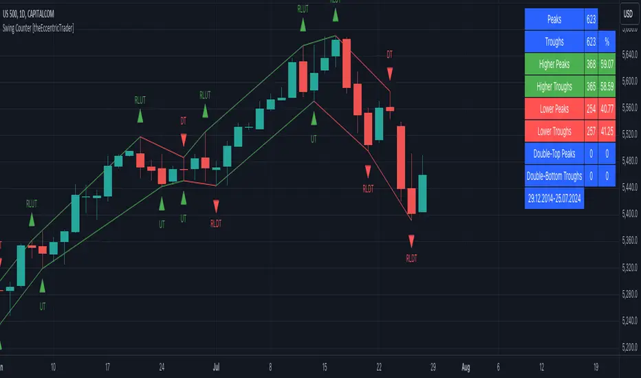
Larry Williams Strategies IndicatorThis indicator is a trend following indicator. It plots some of the trend following strategies described by Larry Williams in his book 'Long Term Secrets to Short Term Trading'. Below are types of trend following strategies you can trade using this indicator. These are notes taken directly from Larry Williams' book.
Short Term Low Strategy
Short Term Low - Any daily low with higher lows on each side of it.
Intermediate Term Low – Any short term low with higher short term lows on each side of it.
Long Term Low – Any intermediate term low with higher intermediate term lows on each side of it.
Conceptual pattern for best buying opportunity is when forming an intermediate term low higher than the last intermediate term low.
This setup can be used on all time frames. However since Larry Williams usually trades the daily chart, the daily chart is probably the best timeframe to trade using this strategy.
Entry point – High of the day that has a higher high on the right side of it.
(My interpretation: price crossing above the high of the previous day is the buy signal)
Target – Markets have a strong tendency to rally above the last intermediate term high by the same amount it moved from the last intermediate term high to the lowest point prior to advancing to new highs.
Trailing Stop – Set stop to most recent short term low, move up as new short term lows are formed. Can also use formation of next intermediate term high as an exit point.
A 'run' to the upside is over when price fails to move higher the next day and falls below the prior day's low.
Short Term High Strategy
Short Term High - Any daily high with lower highs on each side of it.
Intermediate Term High – Any short term high with lower short term highs on each side of it.
Long Term High – Any intermediate term high with lower intermediate term highs on each side of it.
Conceptual pattern for best selling opportunity is when forming an intermediate term high lower than the last intermediate term high.
This setup can be used on all time frames. However since Larry Williams usually trades the daily chart, the daily chart is probably the best timeframe to trade using this strategy.
Entry point – Low of the day that has a lower low on the right side of it.
(My interpretation: price crossing below the low of the previous day is the sell short signal)
Target – Markets have a strong tendency to fall below the last intermediate term low by the same amount it moved from the last intermediate term low to the highest point prior to declining to new lows.
Trailing Stop – Set stop to most recent short term high, move down as new short term highs are formed. Can also use formation of next intermediate term low as an exit point.
A 'run' to the downside is over when price fails to move lower the next day and rises above the prior day's high.
Trend Reversals
A trend change from down to up occurs when a short term high is exceeded on the upside, a trend change from up to down is identified by price going below the most recent low.
Can take these signals to make trades, but it is best to filter them with a confirmation or edge such as Trading Day of the Week, Trading Day of the Month, trendlines, etc. to cut down on false signals.
Three Bar High/Low System
Calculate a three bar moving average of the highs and a three bar moving average of the lows.
Strategy is to buy at the at the price of the three bar moving average of the lows - if the trend is positive according to the swing point trend identification technique - and take profits at the three bar moving average of the highs.
Selling is just the opposite. Sell short at the three bar moving average of the highs and take profits at the three bar moving average of the lows, using the trend identification technique above for confirmation.
This strategy can work on any timeframe, but was described as a daytrading system by Larry Williams.

Market Structure- Zig Zag, BoS and Supply/Demand Zones LIMITLESS// This Pine Script® code is subject to the terms of the Mozilla Public License 2.0 at mozilla.org
// © The_Forex_Steward
//@version=6
indicator("Market Structure- Zig Zag, BoS and Supply/Demand Zones", overlay=true)
// === User Inputs ===
htf = input.timeframe("", title="Timeframe")
internalShiftMode = input.string("Engulfment", title="Calculate Zig-Zag By", options= )
x = input.int(1, minval=1, maxval= 3, title="# of Candles for Zones (1-3)")
showBearishOrderBlocks = input.bool(true, title="Show Supply Zones")
showBullishOrderBlocks = input.bool(true, title="Show Demand Zones")
orderBlockDuration = input.int(10, title="Zone Duration (bars)")
deleteMitigatedBoxes = input.bool(false, title="Delete Mitigated Zones")
deleteBrokenBoxes= input.bool(true, title = "Delete Broken Zones")
dimMitigatedBoxes = input.bool(true, title="Dim Mitigated Zones")
bearishBlockColor = input.color(color.rgb(255, 82, 82, 50), title="Supply Zone Fill")
bullishBlockColor = input.color(color.rgb(76, 175, 79, 50), title="Demand Zone Fill")
lighterBullishColor = color.new(bullishBlockColor, 85) // More transparent
lighterBearishColor = color.new(bearishBlockColor, 85)
zigzagLineColor = input.color(color.black, title="ZigZag Line Color")
zigzagLineWidth = input.int(2, title="Width of Lines", minval=1, maxval=10)
zigzagLineStyle = input.string("Solid", title="ZigZag Line Style", options= )
internalShiftColor = color.new(zigzagLineColor, 75) // More transparent
bosBullishLineColor = input.color(color.green, title="Bullish BOS Line Color")
bosBearishLineColor = input.color(color.red, title="Bearish BOS Line Color")
bosLineStyle = input.string("Dotted", title="BOS Line Style", options= )
bosLineStyleConst = bosLineStyle == "Solid" ? line.style_solid : bosLineStyle == "Dotted" ? line.style_dotted : line.style_dashed
alertMode = input.string("MTF", title= "Enable/Disable for Any Alert() Function Call↓ Alert Status→", options= )
alertSupplyandDemand = input.bool(true, title= "Supply & Demand Zones")
alertHighsandLows = input.bool(true, title= "Swing Highs & Lows")
alertBoS = input.bool(true, title= "BoS")
alertMS = input.bool(true, title= "Market Shifts")
hhBackgroundColor = color.rgb(76, 175, 79, 100)
hhTextColor = color.green
lhBackgroundColor = color.rgb(0, 137, 123, 100)
lhTextColor = color.red
llBackgroundColor = color.rgb(255, 82, 82, 100)
llTextColor = color.red
hlBackgroundColor = color.rgb(255, 153, 0, 100)
hlTextColor = color.green
HtfOpen = request.security(syminfo.tickerid, htf, open)
HtfHigh = request.security(syminfo.tickerid, htf, high)
HtfLow = request.security(syminfo.tickerid, htf, low)
HtfClose = request.security(syminfo.tickerid, htf, close)
prevHtfHigh = request.security(syminfo.tickerid, htf, high )
prevHtfLow = request.security(syminfo.tickerid, htf, low )
isHTFBarClose = ta.change(HtfClose) != 0
// Track the bar_index of the current bar when HTF closes
var int HtfBarIndex = na
if isHTFBarClose
HtfBarIndex := bar_index
// === Initialization ===
var int lastSignal = 0 // 0 = none, 1 = bull, -1 = bear
var float runningLowestHigh = na
var float runningHighestLow = na
// Track engulfed ranges
var float engulfedHigh = na
var float engulfedLow = na
// === Step 1: Detect "starter" engulfing ===
starterBull = HtfClose < HtfOpen and HtfClose > HtfOpen and HtfClose > HtfHigh
starterBear = HtfClose > HtfOpen and HtfClose < HtfOpen and HtfClose < HtfLow
if lastSignal == 0
if starterBull
lastSignal := 1
runningHighestLow := HtfLow
engulfedHigh := HtfHigh
engulfedLow := HtfLow
else if starterBear
lastSignal := -1
runningLowestHigh := HtfHigh
engulfedHigh := HtfHigh
engulfedLow := HtfLow
// === Step 2: Update running references ===
if lastSignal == -1 // last was bearish → waiting for bullish
runningLowestHigh := na(runningLowestHigh) ? HtfHigh : math.min(runningLowestHigh, HtfHigh)
else if lastSignal == 1 // last was bullish → waiting for bearish
runningHighestLow := na(runningHighestLow) ? HtfLow : math.max(runningHighestLow, HtfLow)
// === Step 3: Check for new engulfment ===
newBull = lastSignal == -1 and not na(runningLowestHigh) and HtfClose > runningLowestHigh
newBear = lastSignal == 1 and not na(runningHighestLow) and HtfClose < runningHighestLow
var int lastBullIndex = na
var int lastBearIndex = na
if newBull
lastBullIndex := HtfBarIndex
// store engulfed candle values (the one we just broke over)
engulfedHigh := runningLowestHigh
engulfedLow := HtfLow // or HtfLow depending on how you define "engulfed"
if newBear
lastBearIndex := HtfBarIndex
engulfedLow := runningHighestLow
engulfedHigh := HtfHigh
// === Step 4: Confirm and flip state ===
if newBull
lastSignal := 1
runningLowestHigh := na
runningHighestLow := HtfLow
else if newBear
lastSignal := -1
runningHighestLow := na
runningLowestHigh := HtfHigh
// === Track Boxes ===
var box bullishBoxes = array.new()
var box bearishBoxes = array.new()
// === Mitigation Flags ===
var bool bullishMitigated = false
var bool bearishMitigated = false
var bool bullishBreak = false
var bool bearishBreak = false
// === Delete invalidated boxes ===
if deleteBrokenBoxes
if array.size(bullishBoxes) > 0
for i = array.size(bullishBoxes) - 1 to 0
boxItem = array.get(bullishBoxes, i)
if HtfClose < box.get_bottom(boxItem)
box.delete(boxItem)
array.remove(bullishBoxes, i)
if array.size(bearishBoxes) > 0
for i = array.size(bearishBoxes) - 1 to 0
boxItem = array.get(bearishBoxes, i)
if HtfClose > box.get_top(boxItem)
box.delete(boxItem)
array.remove(bearishBoxes, i)
// === Delete mitigated boxes (optional) ===
if deleteMitigatedBoxes
if array.size(bullishBoxes) > 0
for i = array.size(bullishBoxes) - 1 to 0
boxItem = array.get(bullishBoxes, i)
if HtfLow < box.get_top(boxItem)
bullishMitigated := true
box.delete(boxItem)
array.remove(bullishBoxes, i)
if array.size(bearishBoxes) > 0
for i = array.size(bearishBoxes) - 1 to 0
boxItem = array.get(bearishBoxes, i)
if HtfHigh > box.get_bottom(boxItem)
bearishMitigated := true
box.delete(boxItem)
array.remove(bearishBoxes, i)
if dimMitigatedBoxes
if array.size(bullishBoxes) > 0
for i = 0 to array.size(bullishBoxes) - 1
boxItem = array.get(bullishBoxes, i)
if HtfLow < box.get_top(boxItem)
bullishMitigated := true
box.set_bgcolor(boxItem, lighterBullishColor)
box.set_border_color(boxItem, lighterBullishColor)
if array.size(bearishBoxes) > 0
for i = 0 to array.size(bearishBoxes) - 1
boxItem = array.get(bearishBoxes, i)
if HtfHigh > box.get_bottom(boxItem)
bearishMitigated := true
box.set_bgcolor(boxItem, lighterBearishColor)
box.set_border_color(boxItem, lighterBearishColor)
// Peramters for boxes
zoneHigh = ta.highest(HtfHigh , x)
zoneLow = ta.lowest(HtfLow , x)
// Create new order blocks with adjusted alignment
if showBullishOrderBlocks and newBull
bullishBox = box.new(left= HtfBarIndex , right=HtfBarIndex + orderBlockDuration, top=zoneHigh, bottom=zoneLow, border_color=bullishBlockColor, bgcolor=bullishBlockColor)
array.push(bullishBoxes, bullishBox)
if showBearishOrderBlocks and newBear
bearishBox = box.new(left= HtfBarIndex , right=HtfBarIndex + orderBlockDuration, top=zoneHigh, bottom=zoneLow, border_color=bearishBlockColor, bgcolor=bearishBlockColor)
array.push(bearishBoxes, bearishBox)
// === Internal Structure Logic ===
var int bullishCount = 0
var int bearishCount = 0
var float lowestBullishPrice = na
var float highestBearishPrice = na
var float firstBullishOpen = na
var float firstBearishOpen = na
var int lastInternalShift = 0
var float lastBullishInternalShiftPrice = na
var float lastBearishInternalShiftPrice = na
var float currentSwingHigh = na
var int currentSwingHighIndex = na
var float currentSwingLow = na
var int currentSwingLowIndex = na
var float prevSwingHigh = na
var float prevSwingLow = na
var bool isHH = false
var bool isHL = false
var bool isLL = false
var bool isLH = false
var bool isLiquiditySweep = false
var float lastOpposingLow = na // For HH
var float lastOpposingHigh = na // For LL
var bool internalShiftBullish = false
var bool internalShiftBearish = false
if ((internalShiftMode == "Engulfment") or (internalShiftMode == "Market Shift (Engulfment)"))
internalShiftBullish := newBull
internalShiftBearish := newBear
allowInternalShiftBearish = internalShiftBearish and lastInternalShift != -1
allowInternalShiftBullish = internalShiftBullish and lastInternalShift != 1
var bool plotBearishInternalShift = false
var bool plotBullishInternalShift = false
// === Determine Internal Shift Based on User Input ===
plotBearishInternalShift := false
plotBullishInternalShift := false
if allowInternalShiftBearish
plotBearishInternalShift := true
lastInternalShift := -1
if allowInternalShiftBullish
plotBullishInternalShift := true
lastInternalShift := 1
// === Plot internal shift markers ==
plotshape(plotBullishInternalShift, title="Bullish Internal Shift", location=location.belowbar, color=internalShiftColor, style=shape.triangleup, size=size.tiny)
plotshape(plotBearishInternalShift, title="Bearish Internal Shift", location=location.abovebar, color=internalShiftColor, style=shape.triangledown, size=size.tiny)
// === Highest High Between Alternate Bearish Break and Last Bullish Break (Safe) ===
var float localHigh = na
var int localHighIndex = na
maxHistory = 10000
if plotBearishInternalShift and ((internalShiftMode == "Engulfment") or (internalShiftMode == "Market Shift (Engulfment)"))
float highestHigh = na
int highestIndex = na
int startIndex = math.max(lastBullIndex, bar_index - maxHistory)
int endIndex = HtfBarIndex
for i = startIndex to endIndex
int lookback = bar_index - i // Convert i to relative offset for series access
if lookback >= 0 and lookback < maxHistory and not na(HtfHigh )
if na(highestHigh) or HtfHigh > highestHigh
highestHigh := HtfHigh
highestIndex := i
localHigh := highestHigh
localHighIndex := highestIndex
// === Lowest Low Between Alternate Bullish Break and Last Bearish Break (Safe) ===
var float localLow = na
var int localLowIndex = na
if plotBullishInternalShift and ((internalShiftMode == "Engulfment") or (internalShiftMode == "Market Shift (Engulfment)"))
float lowestLow = na
int lowestIndex = na
int startIndex = math.max(lastBearIndex, HtfBarIndex - maxHistory)
int endIndex = bar_index
for i = startIndex to endIndex
int lookback = bar_index - i // Convert i to relative offset
if lookback >= 0 and lookback < maxHistory and not na(HtfLow )
if na(lowestLow) or HtfLow < lowestLow
lowestLow := HtfLow
lowestIndex := i
localLow := lowestLow
localLowIndex := lowestIndex
// === Track Last Non-Alternating Break of Structure (BoS) ===
var int lastBullishBoSBarNA = na
var int lastBearishBoSBarNA = na
var float lastBullishBoSPriceNA = na
var float lastBearishBoSPriceNA = na
var bool bullishBOSOccurred = false
var bool bearishBOSOccurred = false
var int lastLowIndex = na
var int lastHighIndex = na
var float lastSwingHigh = na
var float lastSwingLow = na
// Reset flags
var bool canBreakBullish = true
var bool canBreakBearish = true
// BoS Conditions (non-alternating)
bullishBoS = canBreakBullish and HtfOpen < localHigh and HtfClose > localHigh
bearishBoS = canBreakBearish and HtfOpen > localLow and HtfClose < localLow
if bullishBoS and internalShiftMode == "Engulfment"
lastBullishBoSBarNA := bar_index
lastBullishBoSPriceNA := HtfClose
canBreakBullish := false // prevent further BoS on same localHigh
bullishBOSOccurred := true
line.new(x1=localHighIndex, y1=localHigh, x2=bar_index, y2=localHigh, color=bosBullishLineColor, width=zigzagLineWidth, style=bosLineStyleConst)
lastSwingHigh := na
if bearishBoS and internalShiftMode == "Engulfment"
lastBearishBoSBarNA := bar_index
lastBearishBoSPriceNA := HtfClose
canBreakBearish := false // prevent further BoS on same localLow
bearishBOSOccurred := true
line.new(x1=localLowIndex, y1=localLow, x2=bar_index, y2=localLow, color=bosBearishLineColor, width=zigzagLineWidth, style=bosLineStyleConst)
lastSwingLow := na
// Reset logic — allow new break only if local high/low changes
if ta.change(localHigh) != 0
canBreakBullish := true
if ta.change(localLow) != 0
canBreakBearish := true
// === Track Last MS Event ===
var int lastBullishBoSBar = na
var int lastBearishBoSBar = na
var float lastBullishBoSPrice = na
var float lastBearishBoSPrice = na
var bool SwingHighBOSOccurred = false
var bool SwingLowBOSOccurred = false
var int lastSwingLowIndex = na
var int lastSwingHighIndex = na
var float lastSSwingHigh = na
var float lastSSwingLow = na
// Track last BoS type: 1 = bullish, -1 = bearish, 0 = none yet
var int lastBoSType = 0
// === Track Last MS Type ===
var int lastMSType = na // 1 = bullish, -1 = bearish
// === MS Detection Logic ===
rawBullishMS = HtfClose > localHigh
rawBearishMS = HtfClose < localLow
// === Enforce Alternation ===
canBullishMS = na(lastMSType) or lastMSType == -1
canBearishMS = na(lastMSType) or lastMSType == 1
bullishMS = rawBullishMS and canBullishMS
bearishMS = rawBearishMS and canBearishMS
plotshape(bullishMS, title="Bullish Market Shift", location=location.belowbar, color=zigzagLineColor, style=shape.triangleup, size=size.tiny)
plotshape(bearishMS, title="Bearish Market Shift", location=location.abovebar, color=zigzagLineColor, style=shape.triangledown, size=size.tiny)
// === Update Last MS Type and BoS Bars ===
if bullishMS
lastMSType := 1
lastBullishBoSBar := bar_index
if bearishMS
lastMSType := -1
lastBearishBoSBar := bar_index
// === Lowest Low Between Last Bearish MS and This Bullish MS ===
var float msLocalLow = na
var int msLocalLowIndex = na
msMaxHistory = 5000
if bullishMS
float msLowestLow = na
int msLowestIndex = na
int msStartIndex = na(lastBearishBoSBar) ? bar_index - msMaxHistory : lastBearishBoSBar
int msEndIndex = bar_index // safer than using HtfBarIndex unless defined
for i = msStartIndex to msEndIndex
int msLookback = bar_index - i
if msLookback >= 0 and msLookback < msMaxHistory and not na(HtfLow )
if na(msLowestLow) or HtfLow < msLowestLow
msLowestLow := HtfLow
msLowestIndex := i
msLocalLow := msLowestLow
msLocalLowIndex := msLowestIndex
// === Highest High Between Last Bullish MS and This Bearish MS ===
var float msLocalHigh = na
var int msLocalHighIndex = na
if bearishMS
float msHighestHigh = na
int msHighestIndex = na
int msStartIndex = na(lastBullishBoSBar) ? bar_index - msMaxHistory : lastBullishBoSBar
int msEndIndex = bar_index
for i = msStartIndex to msEndIndex
int msLookback = bar_index - i
if msLookback >= 0 and msLookback < msMaxHistory and not na(HtfHigh )
if na(msHighestHigh) or HtfHigh > msHighestHigh
msHighestHigh := HtfHigh
msHighestIndex := i
msLocalHigh := msHighestHigh
msLocalHighIndex := msHighestIndex
// === Persistent variables for multiple line handling ===
var line zigzagLines = array.new()
var int lastBearishShiftBar = na
var int lastBullishShiftBar = na
var float lastZigzagPrice = na
var string lastSwingType = ""
// Save shift bar indices
if plotBearishInternalShift
lastBearishShiftBar := bar_index
if plotBullishInternalShift
lastBullishShiftBar := bar_index
// Bearish shift followed by Bullish shift → Track lowest low
if plotBullishInternalShift and internalShiftMode == "Engulfment"
// Plot zigzag line
// Plot zigzag line for LL and HL separately
if not na(prevSwingLow)
if localLow < prevSwingLow // LL
if zigzagLineStyle == "Solid"
line.new(x1=localHighIndex, y1=localHigh, x2=localLowIndex, y2=localLow, color=zigzagLineColor, width=zigzagLineWidth, style=line.style_solid)
else if zigzagLineStyle == "Dotted"
line.new(x1=localHighIndex, y1=localHigh, x2=localLowIndex, y2=localLow, color=zigzagLineColor, width=zigzagLineWidth, style=line.style_dotted)
else if zigzagLineStyle == "Dashed"
line.new(x1=localHighIndex, y1=localHigh, x2=localLowIndex, y2=localLow, color=zigzagLineColor, width=zigzagLineWidth, style=line.style_dashed)
else // LH
if zigzagLineStyle == "Solid"
line.new(x1=localHighIndex, y1=localHigh, x2=localLowIndex, y2=localLow, color=zigzagLineColor, width=zigzagLineWidth, style=line.style_solid)
else if zigzagLineStyle == "Dotted"
line.new(x1=localHighIndex, y1=localHigh, x2=localLowIndex, y2=localLow, color=zigzagLineColor, width=zigzagLineWidth, style=line.style_dotted)
else if zigzagLineStyle == "Dashed"
line.new(x1=localHighIndex, y1=localHigh, x2=localLowIndex, y2=localLow, color=zigzagLineColor, width=zigzagLineWidth, style=line.style_dashed)
// Update swing low and plot label (HL or LL)
if not na(prevSwingLow)
isLL := not na(prevSwingLow) and localLow < prevSwingLow
isHL := not na(prevSwingLow) and localLow > prevSwingLow
if isLL
if bearishBOSOccurred
label.new(localLowIndex, localLow, "LL", color=llBackgroundColor, style=label.style_label_up, textcolor=llTextColor, size=size.small)
isLiquiditySweep := false // Definitely not a sweep if BOS occurred
else
label.new(localLowIndex, localLow, "LS", color=color.rgb(155, 39, 176, 100), style=label.style_label_up, textcolor=color.orange, size=size.small)
isLiquiditySweep := true
else
isLiquiditySweep := false // Reset only if not LL
lastOpposingHigh := prevSwingHigh
bearishBOSOccurred := false
if isHL
label.new(localLowIndex, localLow, "HL", color=hlBackgroundColor, style=label.style_label_up, textcolor=hlTextColor, size=size.small)
lastOpposingHigh := prevSwingHigh
bearishBOSOccurred := false
prevSwingLow := localLow
lastZigzagPrice := localLow
lastSwingLow := localLow
lastLowIndex := localLowIndex
lastBearishShiftBar := bar_index
if bullishMS and internalShiftMode == "Market Shift (Engulfment)"
// Plot zigzag line
// Plot zigzag line for LL and HL separately
if not na(prevSwingLow)
if msLocalLow < prevSwingLow // LL
if zigzagLineStyle == "Solid"
line.new(x1=msLocalHighIndex, y1=msLocalHigh, x2=msLocalLowIndex, y2=msLocalLow, color=zigzagLineColor, width=zigzagLineWidth, style=line.style_solid)
else if zigzagLineStyle == "Dotted"
line.new(x1=msLocalHighIndex, y1=msLocalHigh, x2=msLocalLowIndex, y2=msLocalLow, color=zigzagLineColor, width=zigzagLineWidth, style=line.style_dotted)
else if zigzagLineStyle == "Dashed"
line.new(x1=msLocalHighIndex, y1=msLocalHigh, x2=msLocalLowIndex, y2=msLocalLow, color=zigzagLineColor, width=zigzagLineWidth, style=line.style_dashed)
else // LH
if zigzagLineStyle == "Solid"
line.new(x1=msLocalHighIndex, y1=msLocalHigh, x2=msLocalLowIndex, y2=msLocalLow, color=zigzagLineColor, width=zigzagLineWidth, style=line.style_solid)
else if zigzagLineStyle == "Dotted"
line.new(x1=msLocalHighIndex, y1=msLocalHigh, x2=msLocalLowIndex, y2=msLocalLow, color=zigzagLineColor, width=zigzagLineWidth, style=line.style_dotted)
else if zigzagLineStyle == "Dashed"
line.new(x1=msLocalHighIndex, y1=msLocalHigh, x2=msLocalLowIndex, y2=msLocalLow, color=zigzagLineColor, width=zigzagLineWidth, style=line.style_dashed)
// Update swing low and plot label (HL or LL)
if not na(prevSwingLow)
isLL := not na(prevSwingLow) and msLocalLow < prevSwingLow
isHL := not na(prevSwingLow) and msLocalLow > prevSwingLow
if isLL
label.new(msLocalLowIndex, msLocalLow, "LL", color=llBackgroundColor, style=label.style_label_up, textcolor=llTextColor, size=size.small)
if isHL
label.new(msLocalLowIndex, msLocalLow, "HL", color=hlBackgroundColor, style=label.style_label_up, textcolor=hlTextColor, size=size.small)
lastOpposingHigh := prevSwingHigh
SwingLowBOSOccurred := false
prevSwingLow := msLocalLow
lastZigzagPrice := msLocalLow
lastSwingLow := msLocalLow
lastLowIndex := msLocalLowIndex
lastBearishShiftBar := bar_index
//========================================================================================
if plotBearishInternalShift and internalShiftMode == "Engulfment"
// Plot zigzag line
if not na(prevSwingHigh)
if localHigh > prevSwingHigh // HH
if zigzagLineStyle == "Solid"
line.new(x1=localLowIndex, y1=localLow, x2=localHighIndex, y2=localHigh, color=zigzagLineColor, width=zigzagLineWidth, style=line.style_solid)
else if zigzagLineStyle == "Dotted"
line.new(x1=localLowIndex, y1=localLow, x2=localHighIndex, y2=localHigh, color=zigzagLineColor, width=zigzagLineWidth, style=line.style_dotted)
else if zigzagLineStyle == "Dashed"
line.new(x1=localLowIndex, y1=localLow, x2=localHighIndex, y2=localHigh, color=zigzagLineColor, width=zigzagLineWidth, style=line.style_dashed)
else // LH
if zigzagLineStyle == "Solid"
line.new(x1=localLowIndex, y1=localLow, x2=localHighIndex, y2=localHigh, color=zigzagLineColor, width=zigzagLineWidth, style=line.style_solid)
else if zigzagLineStyle == "Dotted"
line.new(x1=localLowIndex, y1=localLow, x2=localHighIndex, y2=localHigh, color=zigzagLineColor, width=zigzagLineWidth, style=line.style_dotted)
else if zigzagLineStyle == "Dashed"
line.new(x1=localLowIndex, y1=localLow, x2=localHighIndex, y2=localHigh, color=zigzagLineColor, width=zigzagLineWidth, style=line.style_dashed)
// Update swing high and plot label (HH or LH)
if not na(prevSwingHigh)
isHH := not na(prevSwingHigh) and localHigh > prevSwingHigh
isLH := not na(prevSwingHigh) and localHigh < prevSwingHigh
if isHH
if bullishBOSOccurred
label.new(localHighIndex, localHigh, "HH", color=hhBackgroundColor, style=label.style_label_down, textcolor=hhTextColor, size=size.small)
isLiquiditySweep := false
else
label.new(localHighIndex, localHigh, "LS", color=color.rgb(155, 39, 176, 100), style=label.style_label_down, textcolor=color.orange, size=size.small)
isLiquiditySweep := true
else
isLiquiditySweep := false
bullishBOSOccurred := false
if isLH
label.new(localHighIndex, localHigh, "LH", color=lhBackgroundColor, style=label.style_label_down, textcolor=lhTextColor, size=size.small)
lastOpposingLow := prevSwingLow
bullishBOSOccurred := false
prevSwingHigh := localHigh
lastZigzagPrice := localHigh
lastSwingHigh := localHigh
lastHighIndex := localHighIndex
lastBullishShiftBar := bar_index
if bearishMS and internalShiftMode == "Market Shift (Engulfment)"
// Plot zigzag line
if not na(prevSwingHigh)
if msLocalHigh > prevSwingHigh // HH
if zigzagLineStyle == "Solid"
line.new(x1=msLocalLowIndex, y1=msLocalLow, x2=msLocalHighIndex, y2=msLocalHigh, color=zigzagLineColor, width=zigzagLineWidth, style=line.style_solid)
else if zigzagLineStyle == "Dotted"
line.new(x1=msLocalLowIndex, y1=msLocalLow, x2=msLocalHighIndex, y2=msLocalHigh, color=zigzagLineColor, width=zigzagLineWidth, style=line.style_dotted)
else if zigzagLineStyle == "Dashed"
line.new(x1=msLocalLowIndex, y1=msLocalLow, x2=msLocalHighIndex, y2=msLocalHigh, color=zigzagLineColor, width=zigzagLineWidth, style=line.style_dashed)
else // LH
if zigzagLineStyle == "Solid"
line.new(x1=msLocalLowIndex, y1=msLocalLow, x2=msLocalHighIndex, y2=msLocalHigh, color=zigzagLineColor, width=zigzagLineWidth, style=line.style_solid)
else if zigzagLineStyle == "Dotted"
line.new(x1=msLocalLowIndex, y1=msLocalLow, x2=msLocalHighIndex, y2=msLocalHigh, color=zigzagLineColor, width=zigzagLineWidth, style=line.style_dotted)
else if zigzagLineStyle == "Dashed"
line.new(x1=msLocalLowIndex, y1=msLocalLow, x2=msLocalHighIndex, y2=msLocalHigh, color=zigzagLineColor, width=zigzagLineWidth, style=line.style_dashed)
// Update swing high and plot label (HH or LH)
if not na(prevSwingHigh)
isHH := not na(prevSwingHigh) and msLocalHigh > prevSwingHigh
isLH := not na(prevSwingHigh) and msLocalHigh < prevSwingHigh
if isHH
label.new(msLocalHighIndex, msLocalHigh, "HH", color=hhBackgroundColor, style=label.style_label_down, textcolor=hhTextColor, size=size.small)
SwingHighBOSOccurred := false
if isLH
label.new(msLocalHighIndex, msLocalHigh, "LH", color=lhBackgroundColor, style=label.style_label_down, textcolor=lhTextColor, size=size.small)
lastOpposingLow := prevSwingLow
SwingHighBOSOccurred := false
prevSwingHigh := msLocalHigh
lastZigzagPrice := msLocalHigh
lastSwingHigh := msLocalHigh
lastHighIndex := msLocalHighIndex
lastBullishShiftBar := bar_index
// === Alert Conditions ===
alertcondition(newBull, title="New Supply Zone", message="New supply zone available.")
alertcondition(newBear, title="New Demand Zone", message="New demand zone available.")
alertcondition(plotBullishInternalShift, title="Bullish Internal Shift (All Lows)", message="Bullish Internal Shift detected! Check Swing Low.")
alertcondition(plotBearishInternalShift, title="Bearish Internal Shift (All Highs)", message="Bearish Internal Shift detected! Check Swing High.")
alertcondition(bullishBOSOccurred, title="Bullish Break of Structure", message="Bullish BoS detected.")
alertcondition(bearishBOSOccurred, title="Bearish Break of Structure", message="Bearish BoS detected.")
alertcondition(bullishMS, title="Bullish Market Shift", message="Bullish market shift detected.")
alertcondition(bearishMS, title="Bearish Market Shift", message="Bearish market shift detected.")
alertcondition(isHH and plotBearishInternalShift and not isLiquiditySweep, title="Higher High (HH)", message="Higher High (HH) detected")
alertcondition(isHL and plotBullishInternalShift, title="Higher Low (HL)", message="Higher Low (HL) detected")
alertcondition(isLL and plotBullishInternalShift and not isLiquiditySweep, title="Lower Low (LL)", message="Lower Low (LL) detected")
alertcondition(isLH and plotBearishInternalShift, title="Lower High (LH)", message="Lower High (LH) detected")
alertcondition((isLiquiditySweep and isLL and plotBullishInternalShift) or (isLiquiditySweep and isHH and plotBearishInternalShift), title="Liquidity Sweep (LS)", message="Liquidity Sweep (LS) detected")
// === Alerts ===
if alertMode == "LTF"
if isHH and plotBearishInternalShift and not isLiquiditySweep and (alertHighsandLows == true)
alert("Higher High (HH) detected (LTF)", alert.freq_once_per_bar_close)
if isHL and plotBullishInternalShift and (alertHighsandLows == true)
alert("Higher Low (HL) detected (LTF)", alert.freq_once_per_bar_close)
if isLL and plotBullishInternalShift and not isLiquiditySweep and (alertHighsandLows == true)
alert("Lower Low (LL) detected (LTF)" , alert.freq_once_per_bar_close)
if isLH and plotBearishInternalShift and (alertHighsandLows == true)
alert("Lower High (LH) detected (LTF)", alert.freq_once_per_bar_close)
if ((isLiquiditySweep and isLL and plotBullishInternalShift) or (isLiquiditySweep and isHH and plotBearishInternalShift)) and (alertHighsandLows == true)
alert("Liquidity Sweep (LS) detected (LTF)", alert.freq_once_per_bar_close)
if newBear and (alertSupplyandDemand == true)
alert("New supply zone available. (LTF)", alert.freq_once_per_bar_close)
if newBull and (alertSupplyandDemand == true)
alert("New demand zone available. (LTF)", alert.freq_once_per_bar_close)
if bullishBOSOccurred and (alertBoS == true)
alert("Bullish BoS detected. (LTF)", alert.freq_once_per_bar_close)
if bearishBOSOccurred and (alertBoS == true)
alert("Bearish BoS detected. (LTF)", alert.freq_once_per_bar_close)
if bullishMS and (alertMS == true)
alert("Bullish market shift detected (LTF).", alert.freq_once_per_bar_close)
if bearishMS and (alertMS == true)
alert("Bearish market shift detected (LTF).", alert.freq_once_per_bar_close)
if alertMode == "MTF"
if isHH and plotBearishInternalShift and not isLiquiditySweep and (alertHighsandLows == true)
alert("Higher High (HH) detected (MTF)", alert.freq_once_per_bar_close)
if isHL and plotBullishInternalShift and (alertHighsandLows == true)
alert("Higher Low (HL) detected (MTF)", alert.freq_once_per_bar_close)
if isLL and plotBullishInternalShift and not isLiquiditySweep and (alertHighsandLows == true)
alert("Lower Low (LL) detected (MTF)" , alert.freq_once_per_bar_close)
if isLH and plotBearishInternalShift and (alertHighsandLows == true)
alert("Lower High (LH) detected (MTF)", alert.freq_once_per_bar_close)
if ((isLiquiditySweep and isLL and plotBullishInternalShift) or (isLiquiditySweep and isHH and plotBearishInternalShift)) and (alertHighsandLows == true)
alert("Liquidity Sweep (LS) detected (MTF)", alert.freq_once_per_bar_close)
if newBear and (alertSupplyandDemand == true)
alert("New supply zone available. (MTF)", alert.freq_once_per_bar_close)
if newBull and (alertSupplyandDemand == true)
alert("New demand zone available. (MTF)", alert.freq_once_per_bar_close)
if bullishBOSOccurred and (alertBoS == true)
alert("Bullish BoS detected. (MTF)", alert.freq_once_per_bar_close)
if bearishBOSOccurred and (alertBoS == true)
alert("Bearish BoS detected. (MTF)", alert.freq_once_per_bar_close)
if bullishMS and (alertMS == true)
alert("Bullish market shift detected (MTF).", alert.freq_once_per_bar_close)
if bearishMS and (alertMS == true)
alert("Bearish market shift detected (MTF).", alert.freq_once_per_bar_close)
if alertMode == "HTF"
if isHH and plotBearishInternalShift and not isLiquiditySweep and (alertHighsandLows == true)
alert("Higher High (HH) detected (HTF)", alert.freq_once_per_bar_close)
if isHL and plotBullishInternalShift and (alertHighsandLows == true)
alert("Higher Low (HL) detected (HTF)", alert.freq_once_per_bar_close)
if isLL and plotBullishInternalShift and not isLiquiditySweep and (alertHighsandLows == true)
alert("Lower Low (LL) detected (HTF)" , alert.freq_once_per_bar_close)
if isLH and plotBearishInternalShift and (alertHighsandLows == true)
alert("Lower High (LH) detected (HTF)", alert.freq_once_per_bar_close)
if ((isLiquiditySweep and isLL and plotBullishInternalShift) or (isLiquiditySweep and isHH and plotBearishInternalShift)) and (alertHighsandLows == true)
alert("Liquidity Sweep (LS) detected (HTF)", alert.freq_once_per_bar_close)
if newBear and (alertSupplyandDemand == true)
alert("New supply zone available. (HTF)", alert.freq_once_per_bar_close)
if newBull and (alertSupplyandDemand == true)
alert("New demand zone available. (HTF)", alert.freq_once_per_bar_close)
if bullishBOSOccurred and (alertBoS == true)
alert("Bullish BoS detected. (HTF)", alert.freq_once_per_bar_close)
if bearishBOSOccurred and (alertBoS == true)
alert("Bearish BoS detected. (HTF)", alert.freq_once_per_bar_close)
if bullishMS and (alertMS == true)
alert("Bullish market shift detected (HTF).", alert.freq_once_per_bar_close)
if bearishMS and (alertMS == true)
alert("Bearish market shift detected (HTF).", alert.freq_once_per_bar_close)

BBMA By K1M4K-ID- Final Validated Re-Entry//@version=6
indicator("BBMA By K1M4K-ID- Final Validated Re-Entry", overlay=true, max_labels_count=500)
// === INPUT BB ===
lengthBB = input.int(20, title="BB Period")
devBB = input.float(2.0, title="Deviation")
src = input.source(close, title="Source")
bbColorMid = input.color(color.purple, title="Mid BB Color")
bbColorTop = input.color(color.purple, title="Top BB Color")
bbColorLow = input.color(color.purple, title="Low BB Color")
showFill = input.bool(true, title="Show BB Fill")
showReEntrySignals = input.bool(true, "Show Re-Entry Signals (✅)")
showSignalTable = input.bool(true, "Show Signal Table")
// === BB CALCULATION ===
basis = ta.sma(src, lengthBB)
dev = devBB * ta.stdev(src, lengthBB)
topBB = basis + dev
lowBB = basis - dev
// === PLOT BB ===
pMid = plot(basis, title="Mid BB", color=bbColorMid, linewidth=2)
pTop = plot(topBB, title="Top BB", color=bbColorTop, linewidth=2)
pLow = plot(lowBB, title="Low BB", color=bbColorLow, linewidth=2)
fill(pTop, pLow, color=showFill ? color.new(color.purple, 85) : na, title="BB Fill")
// === INPUT MA SETTING ===
ma_func(source, length) => ta.wma(source, length)
// === MA HIGH/LOW ===
ma5_high = ma_func(high, 5)
ma10_high = ma_func(high, 10)
ma5_low = ma_func(low, 5)
ma10_low = ma_func(low, 10)
// === PLOT MA ===
p_ma5_high = plot(ma5_high, title="MA 5 High", color=color.green, linewidth=2)
p_ma10_high = plot(ma10_high, title="MA 10 High", color=color.green, linewidth=2)
fill(p_ma5_high, p_ma10_high, color=color.new(color.green, 85), title="MA High Fill")
p_ma5_low = plot(ma5_low, title="MA 5 Low", color=color.red, linewidth=2)
p_ma10_low = plot(ma10_low, title="MA 10 Low", color=color.red, linewidth=2)
fill(p_ma5_low, p_ma10_low, color=color.new(color.red, 85), title="MA Low Fill")
// === EMA 50 ===
ema50 = ta.ema(close, 50)
plot(ema50, title="EMA 50", color=color.blue, linewidth=3)
// === CSA KUKUH (LOGIKA ASLI LU - TIDAK DIUBAH) ===
var bool hasCsaBuy = false
var bool hasCsaSell = false
isCsaKukuhBuy = close > ma5_high and close > ma10_high and close > basis
isCsaKukuhSell = close < ma5_low and close < ma10_low and close < basis
if isCsaKukuhBuy and not hasCsaBuy
hasCsaBuy := true
hasCsaSell := false
else if isCsaKukuhSell and not hasCsaSell
hasCsaSell := true
hasCsaBuy := false
showCsaBuy = isCsaKukuhBuy and not hasCsaBuy
showCsaSell = isCsaKukuhSell and not hasCsaSell
plotshape(showCsaBuy, title="CSA Kukuh Buy First", location=location.belowbar, color=color.green, style=shape.labelup, text="CSAK", textcolor=color.white, size=size.small)
plotshape(showCsaSell, title="CSA Kukuh Sell First", location=location.abovebar, color=color.red, style=shape.labeldown, text="CSAK", textcolor=color.white, size=size.small)
// === CSM (HANYA SAAT KELUAR DARI DALAM BB) ===
wasInsideBB = (close >= lowBB and close <= topBB )
csmBuySignal = wasInsideBB and close > topBB
csmSellSignal = wasInsideBB and close < lowBB
plotshape(csmBuySignal, title="CSM Buy", location=location.abovebar, color=color.green, style=shape.triangleup, text="CSM", size=size.tiny)
plotshape(csmSellSignal, title="CSM Sell", location=location.belowbar, color=color.red, style=shape.triangledown, text="CSM", size=size.tiny)
// === CSA (BREAKOUT TANPA MELEWATI MID BB) ===
isCsaBuy = close > ma5_high and close > ma10_high and close <= basis
isCsaSell = close < ma5_low and close < ma10_low and close >= basis
plotshape(isCsaBuy, title="CSA Buy", location=location.belowbar, color=color.new(color.green, 60), style=shape.circle, text="CSA", size=size.tiny)
plotshape(isCsaSell, title="CSA Sell", location=location.abovebar, color=color.new(color.red, 60), style=shape.circle, text="CSA", size=size.tiny)
// === EXTREME ===
basis_ext = ta.sma(close, 20)
dev_ext = 2 * ta.stdev(close, 20)
isExtremeBuy() => ta.wma(low, 5) < basis_ext - dev_ext
isExtremeSell() => ta.wma(high, 5) > basis_ext + dev_ext
plotshape(isExtremeBuy(), title="Extreme Buy", location=location.belowbar, color=color.green, style=shape.labelup, text="E", size=size.tiny, textcolor=color.white)
plotshape(isExtremeSell(), title="Extreme Sell", location=location.abovebar, color=color.red, style=shape.labeldown, text="E", size=size.tiny, textcolor=color.white)
// === ZZL MA ===
isZzlBuy = (ma5_high > basis and ma10_high > basis and ma5_low > basis and ma10_low > basis and
(ma5_high <= basis or ma10_high <= basis or ma5_low <= basis or ma10_low <= basis))
isZzlSell = (ma5_high < basis and ma10_high < basis and ma5_low < basis and ma10_low < basis and
(ma5_high >= basis or ma10_high >= basis or ma5_low >= basis or ma10_low >= basis))
var bool zzlBuyShown = false
var bool zzlSellShown = false
if isZzlBuy and not zzlBuyShown
label.new(bar_index, low, "Z", style=label.style_label_up, color=color.green, textcolor=color.white)
zzlBuyShown := true
if not isZzlBuy
zzlBuyShown := false
if isZzlSell and not zzlSellShown
label.new(bar_index, high, "Z", style=label.style_label_down, color=color.red, textcolor=color.white)
zzlSellShown := true
if not isZzlSell
zzlSellShown := false
// ===========================================
// === VALIDASI + RE-ENTRY (H4 & H1) ===
// ===========================================
// --- Ambil data ---
= request.security(syminfo.tickerid, "240", )
wasInside_h4 = request.security(syminfo.tickerid, "240", (close >= (ta.sma(close, lengthBB) - devBB * ta.stdev(close, lengthBB) ) and close <= (ta.sma(close, lengthBB) + devBB * ta.stdev(close, lengthBB) )))
csmBuy_h4 = wasInside_h4 and request.security(syminfo.tickerid, "240", close > (ta.sma(close, lengthBB) + devBB * ta.stdev(close, lengthBB)))
csmSell_h4 = wasInside_h4 and request.security(syminfo.tickerid, "240", close < (ta.sma(close, lengthBB) - devBB * ta.stdev(close, lengthBB)))
csakBuy_h4 = close_h4 > ma5h_h4 and close_h4 > ma10h_h4 and close_h4 > basis_h4
csakSell_h4 = close_h4 < ma5l_h4 and close_h4 < ma10l_h4 and close_h4 < basis_h4
csaBuy_h4 = close_h4 > ma5h_h4 and close_h4 > ma10h_h4 and close_h4 <= basis_h4
csaSell_h4 = close_h4 < ma5l_h4 and close_h4 < ma10l_h4 and close_h4 >= basis_h4
csmBuy_h1 = request.security(syminfo.tickerid, "60", (close >= (ta.sma(close, lengthBB) - devBB * ta.stdev(close, lengthBB) ) and close <= (ta.sma(close, lengthBB) + devBB * ta.stdev(close, lengthBB) )) and close > (ta.sma(close, lengthBB) + devBB * ta.stdev(close, lengthBB)))
csmSell_h1 = request.security(syminfo.tickerid, "60", (close >= (ta.sma(close, lengthBB) - devBB * ta.stdev(close, lengthBB) ) and close <= (ta.sma(close, lengthBB) + devBB * ta.stdev(close, lengthBB) )) and close < (ta.sma(close, lengthBB) - devBB * ta.stdev(close, lengthBB)))
csakBuy_h1 = request.security(syminfo.tickerid, "60", close > ta.wma(high,5) and close > ta.wma(high,10) and close > ta.sma(close, lengthBB))
csakSell_h1 = request.security(syminfo.tickerid, "60", close < ta.wma(low,5) and close < ta.wma(low,10) and close < ta.sma(close, lengthBB))
csaBuy_h1 = request.security(syminfo.tickerid, "60", close > ta.wma(high,5) and close > ta.wma(high,10) and close <= ta.sma(close, lengthBB))
csaSell_h1 = request.security(syminfo.tickerid, "60", close < ta.wma(low,5) and close < ta.wma(low,10) and close >= ta.sma(close, lengthBB))
csmBuy_m15 = request.security(syminfo.tickerid, "15", close > (ta.sma(close, lengthBB) + devBB * ta.stdev(close, lengthBB)))
csmSell_m15 = request.security(syminfo.tickerid, "15", close < (ta.sma(close, lengthBB) - devBB * ta.stdev(close, lengthBB)))
csakBuy_d = request.security(syminfo.tickerid, "D", close > ta.wma(high,5) and close > ta.wma(high,10) and close > ta.sma(close, lengthBB))
csakSell_d = request.security(syminfo.tickerid, "D", close < ta.wma(low,5) and close < ta.wma(low,10) and close < ta.sma(close, lengthBB))
csaBuy_d = request.security(syminfo.tickerid, "D", close > ta.wma(high,5) and close > ta.wma(high,10) and close <= ta.sma(close, lengthBB))
csaSell_d = request.security(syminfo.tickerid, "D", close < ta.wma(low,5) and close < ta.wma(low,10) and close >= ta.sma(close, lengthBB))
// --- Validasi ---
validCsakH4Buy = csakBuy_h4 and ta.highest(csmBuy_h1 ? 1 : 0, 4) == 1
validCsakH4Sell = csakSell_h4 and ta.highest(csmSell_h1 ? 1 : 0, 4) == 1
validCsakH1Buy = csakBuy_h1 and ta.highest(csmBuy_m15 ? 1 : 0, 4) == 1
validCsakH1Sell = csakSell_h1 and ta.highest(csmSell_m15 ? 1 : 0, 4) == 1
validCsmH1Buy = csmBuy_h1 and (csaBuy_h4 or csakBuy_h4) and ta.highest(csmBuy_m15 ? 1 : 0, 4) == 1
validCsmH1Sell = csmSell_h1 and (csaSell_h4 or csakSell_h4) and ta.highest(csmSell_m15 ? 1 : 0, 4) == 1
validCsmH4Buy = csmBuy_h4 and (csaBuy_d or csakBuy_d) and ta.highest(csmBuy_h1 or csmSell_h1 ? 1 : 0, 4) == 1
validCsmH4Sell = csmSell_h4 and (csaSell_d or csakSell_d) and ta.highest(csmBuy_h1 or csmSell_h1 ? 1 : 0, 4) == 1
// --- Re-Entry Area ---
inReEntryBuy = low <= math.max(ma5_low, ma10_low)
inReEntrySell = high >= math.min(ma5_high, ma10_high)
// --- Flag Valid + Hit Detection ---
var bool vCsakH4B = false, vCsakH4S = false
var bool vCsakH1B = false, vCsakH1S = false
var bool vCsmH4B = false, vCsmH4S = false
var bool vCsmH1B = false, vCsmH1S = false
var bool hitCsakH4B = false, hitCsakH4S = false
var bool hitCsakH1B = false, hitCsakH1S = false
var bool hitCsmH4B = false, hitCsmH4S = false
var bool hitCsmH1B = false, hitCsmH1S = false
// Reset hit setiap candle
hitCsakH4B := false
hitCsakH4S := false
hitCsakH1B := false
hitCsakH1S := false
hitCsmH4B := false
hitCsmH4S := false
hitCsmH1B := false
hitCsmH1S := false
// Aktifkan flag saat valid
vCsakH4B := validCsakH4Buy ? true : vCsakH4B
vCsakH4S := validCsakH4Sell ? true : vCsakH4S
vCsakH1B := validCsakH1Buy ? true : vCsakH1B
vCsakH1S := validCsakH1Sell ? true : vCsakH1S
vCsmH4B := validCsmH4Buy ? true : vCsmH4B
vCsmH4S := validCsmH4Sell ? true : vCsmH4S
vCsmH1B := validCsmH1Buy ? true : vCsmH1B
vCsmH1S := validCsmH1Sell ? true : vCsmH1S
// Deteksi & reset saat re-entry
if vCsakH4B and inReEntryBuy
hitCsakH4B := true
vCsakH4B := false
if vCsakH4S and inReEntrySell
hitCsakH4S := true
vCsakH4S := false
if vCsakH1B and inReEntryBuy
hitCsakH1B := true
vCsakH1B := false
if vCsakH1S and inReEntrySell
hitCsakH1S := true
vCsakH1S := false
if vCsmH4B and inReEntryBuy
hitCsmH4B := true
vCsmH4B := false
if vCsmH4S and inReEntrySell
hitCsmH4S := true
vCsmH4S := false
if vCsmH1B and inReEntryBuy
hitCsmH1B := true
vCsmH1B := false
if vCsmH1S and inReEntrySell
hitCsmH1S := true
vCsmH1S := false
// --- Plot Re-Entry ---
//plotshape(showReEntrySignals and hitCsakH4B, location=location.belowbar, color=color.teal, style=shape.labelup, text="✅", size=size.normal)
//plotshape(showReEntrySignals and hitCsakH4S, location=location.abovebar, color=color.orange, style=shape.labeldown, text="✅", size=size.normal)
//plotshape(showReEntrySignals and hitCsakH1B, location=location.belowbar, color=color.green, style=shape.labelup, text="✅", size=size.small)
//plotshape(showReEntrySignals and hitCsakH1S, location=location.abovebar, color=color.red, style=shape.labeldown, text="✅", size=size.small)
//plotshape(showReEntrySignals and hitCsmH1B, location=location.belowbar, color=color.green, style=shape.labelup, text="✅ CSM", size=size.tiny)
//plotshape(showReEntrySignals and hitCsmH1S, location=location.abovebar, color=color.red, style=shape.labeldown, text="✅ CSM", size=size.tiny)
//plotshape(showReEntrySignals and hitCsmH4B, location=location.belowbar, color=color.teal, style=shape.labelup, text="✅ CSM", size=size.tiny)
//plotshape(showReEntrySignals and hitCsmH4S, location=location.abovebar, color=color.orange, style=shape.labeldown, text="✅ CSM", size=size.tiny)
// ===========================================
// === TABEL SIGNAL H1 & H4 (FINAL) ===
// ===========================================
var table sigTable = table.new(position.top_right, 4, 5, border_width=1)
if barstate.islast and showSignalTable
table.cell(sigTable, 0, 0, "TF", text_color=color.white, bgcolor=color.black)
table.cell(sigTable, 1, 0, "Signal", text_color=color.white, bgcolor=color.black)
table.cell(sigTable, 2, 0, "Status", text_color=color.white, bgcolor=color.black)
table.cell(sigTable, 3, 0, "Re-Entry", text_color=color.white, bgcolor=color.black)
table.cell(sigTable, 0, 1, "H4", text_color=color.white, bgcolor=color.black)
table.cell(sigTable, 1, 1, "CSAK Buy", text_color=color.green, bgcolor=color.new(color.green, 90))
table.cell(sigTable, 2, 1, vCsakH4B ? "✅ Valid" : "-", text_color=vCsakH4B ? color.green : color.gray, bgcolor=color.new(vCsakH4B ? color.green : color.gray, 90))
table.cell(sigTable, 3, 1, hitCsakH4B ? "✅ Hit" : "-", text_color=hitCsakH4B ? color.teal : color.gray, bgcolor=color.new(hitCsakH4B ? color.teal : color.gray, 90))
table.cell(sigTable, 0, 2, "H4", text_color=color.white, bgcolor=color.black)
table.cell(sigTable, 1, 2, "CSAK Sell", text_color=color.red, bgcolor=color.new(color.red, 90))
table.cell(sigTable, 2, 2, vCsakH4S ? "✅ Valid" : "-", text_color=vCsakH4S ? color.red : color.gray, bgcolor=color.new(vCsakH4S ? color.red : color.gray, 90))
table.cell(sigTable, 3, 2, hitCsakH4S ? "✅ Hit" : "-", text_color=hitCsakH4S ? color.orange : color.gray, bgcolor=color.new(hitCsakH4S ? color.orange : color.gray, 90))
table.cell(sigTable, 0, 3, "H1", text_color=color.white, bgcolor=color.black)
table.cell(sigTable, 1, 3, "CSM Buy", text_color=color.green, bgcolor=color.new(color.green, 90))
table.cell(sigTable, 2, 3, vCsmH1B ? "✅ Valid" : "-", text_color=vCsmH1B ? color.green : color.gray, bgcolor=color.new(vCsmH1B ? color.green : color.gray, 90))
table.cell(sigTable, 3, 3, hitCsmH1B ? "✅ Hit" : "-", text_color=hitCsmH1B ? color.teal : color.gray, bgcolor=color.new(hitCsmH1B ? color.teal : color.gray, 90))
table.cell(sigTable, 0, 4, "H1", text_color=color.white, bgcolor=color.black)
table.cell(sigTable, 1, 4, "CSM Sell", text_color=color.red, bgcolor=color.new(color.red, 90))
table.cell(sigTable, 2, 4, vCsmH1S ? "✅ Valid" : "-", text_color=vCsmH1S ? color.red : color.gray, bgcolor=color.new(vCsmH1S ? color.red : color.gray, 90))
table.cell(sigTable, 3, 4, hitCsmH1S ? "✅ Hit" : "-", text_color=hitCsmH1S ? color.orange : color.gray, bgcolor=color.new(hitCsmH1S ? color.orange : color.gray, 90))

RSI Fibonacci Flow [JOAT]RSI Fibonacci Flow - Advanced Fibonacci Retracement with RSI Confluence
Introduction
RSI Fibonacci Flow is an open-source overlay indicator that combines automatic Fibonacci retracement levels with RSI momentum analysis to identify high-probability trading zones. The indicator automatically detects swing highs and lows, draws Fibonacci levels, and generates confluence signals when RSI conditions align with key Fibonacci zones.
This indicator is designed for traders who use Fibonacci retracements but want additional confirmation from momentum analysis before entering trades.
Originality and Purpose
This indicator is NOT a simple mashup of RSI and Fibonacci tools. It is an original implementation that creates a synergistic relationship between two complementary analysis methods:
Why Combine RSI with Fibonacci? Fibonacci retracements identify WHERE price might reverse, but they don't tell you WHEN. RSI provides the timing component by showing momentum exhaustion. When price reaches the Golden Zone (50%-61.8%) AND RSI shows oversold conditions, the probability of a successful bounce increases significantly.
Original Confluence Scoring System: The indicator calculates a 0-5 confluence score that weights multiple factors: Golden Zone presence (+2), entry zone presence (+1), RSI extreme alignment (+1), RSI divergence (+1), and strong RSI momentum (+1). This scoring system is original to this indicator.
Automatic Pivot Detection: Unlike manual Fibonacci tools, this indicator automatically detects swing highs and lows using a configurable pivot algorithm, then draws Fibonacci levels accordingly. The pivot detection uses a center-bar comparison method that checks if a bar's high/low is the highest/lowest within the specified depth on both sides.
Dynamic Trend Awareness: The indicator determines trend direction based on pivot sequence (last pivot was high or low) and adjusts Fibonacci orientation accordingly. In uptrends, 0% is at swing low; in downtrends, 0% is at swing high.
Each component serves a specific purpose:
Fibonacci levels identify potential reversal zones based on natural price ratios
RSI provides momentum context to filter out low-probability setups
Confluence scoring quantifies setup quality for position sizing decisions
Automatic pivot detection removes subjectivity from level placement
Core Concept: RSI-Fibonacci Confluence
The most powerful trading setups occur when multiple factors align. RSI Fibonacci Flow identifies these moments by:
Automatically detecting price pivots and drawing Fibonacci levels
Tracking which Fibonacci zone the current price occupies
Monitoring RSI for overbought/oversold conditions
Generating signals when RSI extremes coincide with key Fibonacci levels
Scoring confluence strength on a 0-5 scale
When price reaches the Golden Zone (50%-61.8%) while RSI shows oversold conditions in an uptrend, the probability of a bounce increases significantly.
Fibonacci Levels Explained
The indicator draws nine Fibonacci levels based on the most recent swing:
0% (Swing Low/High): The starting point of the move
23.6%: Shallow retracement - often seen in strong trends
38.2%: First significant support/resistance level
50%: Psychological midpoint of the move
61.8% (Golden Ratio): The most important Fibonacci level
78.6%: Deep retracement - last defense before trend failure
100% (Swing High/Low): The end point of the move
127.2% (TP1): First extension target for take profit
161.8% (TP2): Second extension target for take profit
The Golden Zone
The area between 50% and 61.8% is highlighted as the "Golden Zone" because:
It represents the optimal retracement depth for trend continuation
Institutional traders often place orders in this zone
It offers favorable risk-to-reward ratios
Price frequently bounces from this area in healthy trends
When price enters the Golden Zone, the indicator highlights it with a semi-transparent box and optional background coloring.
Pivot Detection System
The indicator uses a configurable pivot detection algorithm:
pivotDetect(float src, int len, bool isHigh) =>
int halfLen = len / 2
float centerVal = nz(src , src)
bool isPivot = true
for i = 0 to len - 1
if isHigh
if nz(src , src) > centerVal
isPivot := false
break
else
if nz(src , src) < centerVal
isPivot := false
break
isPivot ? centerVal : float(na)
This identifies swing highs and lows by checking if a bar's high/low is the highest/lowest within the specified depth on both sides.
Visual Components
1. Fibonacci Lines
Horizontal lines at each Fibonacci level:
Solid lines for major levels (0%, 50%, 61.8%, 100%)
Dashed lines for secondary levels (23.6%, 38.2%, 78.6%)
Dotted lines for extension levels (127.2%, 161.8%)
Color-coded for easy identification
Configurable line width
2. Fibonacci Labels
Price labels at each level showing:
Fibonacci percentage
Actual price at that level
Golden Zone label highlighted
TP1 and TP2 labels for targets
3. Golden Zone Box
A semi-transparent box highlighting the 50%-61.8% zone:
Gold colored border and fill
Extends from swing start to current bar (or beyond if extended)
Provides clear visual of the optimal entry zone
4. ZigZag Lines
Connecting lines between detected pivots:
Cyan for moves from low to high
Orange for moves from high to low
Helps visualize market structure
Configurable line width
5. Pivot Markers
Small labels at detected swing points:
"HH" (Higher High) at swing highs
"LL" (Lower Low) at swing lows
Helps track market structure
6. Entry Signals
BUY and SELL labels when confluence conditions are met:
BUY: RSI oversold + price in entry zone + uptrend + positive momentum
SELL: RSI overbought + price in entry zone + downtrend + negative momentum
Labels include "RSI+FIB" to indicate confluence
Confluence Scoring System
The indicator calculates a confluence score from 0 to 5:
+2 points: Price is in the Golden Zone (50%-61.8%)
+1 point: Price is in the entry zone (38.2%-61.8%)
+1 point: RSI is oversold in uptrend OR overbought in downtrend
+1 point: RSI divergence detected (bullish or bearish)
+1 point: Strong RSI momentum (change > 2 points)
Confluence ratings:
STRONG (4-5): Multiple factors align - high probability setup
MODERATE (2-3): Some factors align - proceed with caution
WEAK (0-1): Few factors align - wait for better setup
Dashboard Panel
The 10-row dashboard provides comprehensive analysis:
RSI Value: Current RSI reading (large text)
RSI State: OVERBOUGHT, OVERSOLD, BULLISH, BEARISH, or NEUTRAL
Fib Trend: UPTREND or DOWNTREND based on last pivot sequence
Price Zone: Current Fibonacci zone (e.g., "GOLDEN ZONE", "38.2% - 50%")
Price: Current close price (large text)
Confluence: Score rating with numeric value (e.g., "STRONG (4/5)")
Nearest Fib: Closest key Fibonacci level with price
TP1 (127.2%): First take profit target price
TP2 (161.8%): Second take profit target price
Input Parameters
Pivot Detection:
Pivot Depth: Bars to look back for swing detection (default: 10)
Min Deviation %: Minimum price move to confirm pivot (default: 1.0)
RSI Settings:
RSI Length: Period for RSI calculation (default: 14)
Source: Price source (default: close)
Overbought: Upper threshold (default: 70)
Oversold: Lower threshold (default: 30)
Fibonacci Display:
Show Fib Lines: Toggle Fibonacci lines (default: enabled)
Show Fib Labels: Toggle price labels (default: enabled)
Show Golden Zone Box: Toggle zone highlight (default: enabled)
Line Width: Thickness of Fibonacci lines (default: 2)
Extend Fib Lines: Extend lines into future (default: enabled)
ZigZag:
Show ZigZag: Toggle connecting lines (default: enabled)
ZigZag Width: Line thickness (default: 2)
Signals:
Show Entry Signals: Toggle BUY/SELL labels (default: enabled)
Show TP Levels: Toggle take profit in dashboard (default: enabled)
Show RSI-Fib Confluence: Toggle confluence analysis (default: enabled)
Dashboard:
Show Dashboard: Toggle information panel (default: enabled)
Position: Choose corner placement
Colors:
Bullish: Color for bullish elements (default: cyan)
Bearish: Color for bearish elements (default: orange)
Neutral: Color for neutral elements (default: gray)
Golden Zone: Color for Golden Zone highlight (default: gold)
How to Use RSI Fibonacci Flow
Identifying Entry Zones:
Wait for price to retrace to the 38.2%-61.8% zone
Check if RSI is approaching oversold (for longs) or overbought (for shorts)
Look for STRONG confluence rating in the dashboard
Enter when BUY or SELL signal appears
Setting Take Profit Targets:
TP1 at 127.2% extension for conservative target
TP2 at 161.8% extension for aggressive target
Consider scaling out at each level
Using the Price Zone:
"BELOW 23.6%" - Price hasn't retraced much; wait for deeper pullback
"23.6% - 38.2%" - Shallow retracement; strong trend continuation possible
"38.2% - 50%" - Good entry zone for trend trades
"GOLDEN ZONE" - Optimal entry zone; highest probability
"61.8% - 78.6%" - Deep retracement; trend may be weakening
"78.6% - 100%" - Very deep; trend reversal possible
"ABOVE/BELOW 100%" - Trend has likely reversed
Confluence Trading Strategy:
Only take trades with confluence score of 3 or higher
STRONG confluence (4-5) warrants larger position size
MODERATE confluence (2-3) warrants smaller position size
WEAK confluence (0-1) - wait for better setup
Alert Conditions
Ten alert conditions are available:
RSI-Fib BUY Signal: Strong bullish confluence detected
RSI-Fib SELL Signal: Strong bearish confluence detected
Price in Golden Zone: Price enters 50%-61.8% zone
New Pivot High: Swing high detected
New Pivot Low: Swing low detected
RSI Overbought: RSI crosses above overbought threshold
RSI Oversold: RSI crosses below oversold threshold
Bullish Divergence: Potential bullish RSI divergence
Bearish Divergence: Potential bearish RSI divergence
Strong Confluence: Confluence score reaches 4 or higher
Understanding Trend Direction
The indicator determines trend based on pivot sequence:
UPTREND: Last pivot was a low after a high (expecting move up)
DOWNTREND: Last pivot was a high after a low (expecting move down)
Fibonacci levels are drawn accordingly:
In uptrend: 0% at swing low, 100% at swing high
In downtrend: 0% at swing high, 100% at swing low
Bar Coloring
When confluence features are enabled:
Cyan bars on strong bullish signals
Orange bars on strong bearish signals
Gold-tinted bars when price is in Golden Zone
Best Practices
Use on 1H timeframe or higher for more reliable pivots
Adjust Pivot Depth based on timeframe (higher for longer timeframes)
Wait for price to enter Golden Zone before considering entries
Confirm RSI is in favorable territory before trading
Use extension levels (127.2%, 161.8%) for realistic profit targets
Combine with support/resistance and candlestick patterns
Higher confluence scores indicate higher probability setups
Limitations
Pivot detection has inherent lag (must wait for confirmation)
Fibonacci levels are subjective - different swings produce different levels
Works best in trending markets with clear swings
RSI can remain overbought/oversold in strong trends
Not all Golden Zone entries will be successful
The source code is open and available for review and modification.
Disclaimer
This indicator is provided for educational and informational purposes only. It is not financial advice. Trading involves substantial risk of loss. Past performance does not guarantee future results. Fibonacci levels are not guaranteed support/resistance - they are probability zones based on historical price behavior. Always conduct your own analysis and use proper risk management.
- Made with passion by officialjackofalltrades :D

[GYTS] Volatility Toolkit Volatility Toolkit
🌸 Part of GoemonYae Trading System (GYTS) 🌸
🌸 --------- INTRODUCTION --------- 🌸
💮 What is Volatility Toolkit?
Volatility Toolkit is a comprehensive volatility analysis indicator featuring academically-grounded range-based estimators. Unlike simplistic measures like ATR, these estimators extract maximum information from OHLC data — resulting in estimates that are 5-14× more statistically efficient than traditional close-to-close methods.
The indicator provides two configurable estimator slots, weighted aggregation, adaptive threshold detection, and regime identification — all with flexible smoothing options via
GYTS FiltersToolkit integration.
💮 Why Use This Indicator?
Standard volatility measures (like simple standard deviation) are highly inefficient, requiring large amounts of data to produce stable estimates. Academic research has shown that range-based estimators extract far more information from the same price data:
• Statistical Efficiency — Yang-Zhang achieves up to 14× the efficiency of close-to-close variance, meaning you can achieve the same estimation accuracy with far fewer bars
• Drift Independence — Rogers-Satchell and Yang-Zhang correctly isolate variance even in strongly trending markets where simpler estimators become biased
• Gap Handling — Yang-Zhang properly accounts for overnight gaps, critical for equity markets
• Regime Detection — Built-in threshold modes identify when volatility enters elevated or suppressed states
↑ Overview showing Yang-Zhang volatility with dynamic threshold bands and regime background colouring
🌸 --------- HOW IT WORKS --------- 🌸
💮 Core Concept
The toolkit groups volatility estimators by their output scale to ensure valid comparisons and aggregations:
• Log-Return Scale (σ) — Close-to-Close, Parkinson, Garman-Klass, Rogers-Satchell, Yang-Zhang. These are comparable and can be aggregated. Annualisable via √(periods_per_year) scaling.
• Price Unit Scale ($) — ATR. Measures volatility in absolute price terms, directly usable for stop-loss placement.
• Percentage Scale (%) — Chaikin Volatility. Measures the rate of change of the trading range — whether volatility is expanding or contracting.
Only estimators with the same scale can be meaningfully compared or aggregated. The indicator enforces this and warns when mixing incompatible scales.
💮 Range-Based Estimator Overview
Range-based estimators utilise High, Low, Open, and Close prices to extract significantly more information about the underlying diffusion process than close-only methods:
• Parkinson (1980) — Uses High-Low range. ~5× more efficient than close-to-close. Assumes zero drift.
• Garman-Klass (1980) — Incorporates Open and Close. ~7.4× more efficient. Assumes zero drift, no gaps.
• Rogers-Satchell (1991) — Drift-independent. Superior in trending markets where Parkinson/GK become biased.
• Yang-Zhang (2000) — Composite estimator handling both drift and overnight gaps. Up to 14× more efficient.
💮 Theoretical Background
• Parkinson, M. (1980). The Extreme Value Method for Estimating the Variance of the Rate of Return. Journal of Business, 53 (1), 61–65. DOI
• Garman, M.B. & Klass, M.J. (1980). On the Estimation of Security Price Volatilities from Historical Data. Journal of Business, 53 (1), 67–78. DOI
• Rogers, L.C.G. & Satchell, S.E. (1991). Estimating Variance from High, Low and Closing Prices. Annals of Applied Probability, 1 (4), 504–512. DOI
• Yang, D. & Zhang, Q. (2000). Drift-Independent Volatility Estimation Based on High, Low, Open, and Close Prices. Journal of Business, 73 (3), 477–491. DOI
🌸 --------- KEY FEATURES --------- 🌸
💮 Feature Reference
Estimators (8 options across 3 scale groups):
• Close-to-Close — Classical benchmark using closing prices only. Least efficient but useful as baseline. Log-return scale.
• Parkinson — Range-based (High-Low), ~5× more efficient than close-to-close. Assumes zero drift. Log-return scale.
• Garman-Klass — OHLC-optimised, ~7.4× more efficient. Assumes zero drift, no gaps. Log-return scale.
• Rogers-Satchell — Drift-independent, handles trending markets where Parkinson/GK become biased. Log-return scale.
• Yang-Zhang — Gap-aware composite, most comprehensive (up to 14× efficient). Uses internal rolling variance (unsmoothed). Log-return scale.
• Std Dev — Standard deviation of log returns. Log-return scale.
• ATR — Average True Range in absolute price units. Useful for stop-loss placement. Price unit scale.
• Chaikin — Rate of change of range. Measures volatility expansion/contraction, not level. Percentage scale.
Smoothing Filters (10 options via FiltersToolkit):
• SMA / EMA — Classical moving averages
• Super Smoother (2-Pole / 3-Pole) — Ehlers IIR filter with excellent noise reduction
• Ultimate Smoother (2-Pole / 3-Pole) — Near-zero lag in passband
• BiQuad — Second-order IIR with configurable Q factor
• ADXvma — Adaptive smoothing, flat during ranging periods
• MAMA — MESA Adaptive Moving Average (cycle-adaptive)
• A2RMA — Adaptive Autonomous Recursive MA
Threshold Modes:
• Static — Fixed threshold values you define (e.g., 0.025 annualised)
• Dynamic — Adaptive bands: baseline ± (standard deviation × multiplier)
• Percentile — Threshold at Nth percentile of recent history (e.g., 80th percentile for high)
Visual Features:
• Level-based colour gradient — Line colour shifts with percentile rank (warm = high vol, cool = low vol)
• Fill to zero — Gradient fill intensity proportional to volatility level
• Threshold fills — Intensity-scaled fills when thresholds are breached
• Regime background — Chart background indicates HIGH/NORMAL/LOW volatility state
• Legend table — Displays estimator names, parameters, current values with percentile ranks (P##)
💮 Dual Estimator Slots
Compare two volatility estimators side-by-side. Each slot independently configures:
• Estimator type (8 options across three scale groups)
• Lookback period and smoothing filter
• Colour palette and visual style
This enables direct comparison between estimators (e.g., Yang-Zhang vs Rogers-Satchell) or between different parameterisations of the same estimator.
↑ Yang-Zhang (reddish) and Rogers-Satchell (greenish)
💮 Flexible Smoothing via FiltersToolkit
All estimators (except Yang-Zhang, which uses internal rolling variance) support configurable smoothing through 10 filter types. Using Infinite Impulse Response (IIR) filters instead of SMA avoids the "drop-off artefact" where volatility readings crash when old spikes exit the window.
Example: Same estimator (Parkinson) with different smoothing filters
Add two instances of Volatility Toolkit to your chart:
• Instance 1: Parkinson with SMA smoothing (lookback 14)
• Instance 2: Parkinson with Super Smoother 2-Pole (lookback 14)
Notice how SMA creates sharp drops when volatile bars exit the window, while Super Smoother maintains a gradual transition.
↑ Two Parkinson estimators — SMA (red mono-colour, showing drop-off artefacts) vs Super Smoother (turquoise mono colour, with smooth transitions)
↑ Garman-Klass with BiQuad (orangy) and 2-pole SuperSmoother filters (greenish)
💮 Weighted Aggregation
Combine multiple estimators into a single weighted average. The indicator automatically:
• Validates scale compatibility (only same-scale estimators can be aggregated)
• Normalises weights (so 2:1 means 67%:33%)
• Displays clear warnings when scales differ
Example: Robust volatility estimate
Combine Yang-Zhang (handles gaps) with Rogers-Satchell (handles drift) using equal weights:
• E1: Yang-Zhang (14)
• E2: Rogers-Satchell (14)
• Aggregation: Enabled, weights 1:1
The aggregated line (with "fill to zero" enabled) provides a more robust estimate by averaging two complementary methodologies.
↑ Yang-Zhang + Rogers-Satchell with aggregation line (thicker) showing combined estimate (notice how opening gaps are handled differently)
Example: Trend-weighted aggregation
In strongly trending markets, weight Rogers-Satchell more heavily since it's drift-independent:
• Estimator 1: Garman-Klass (faster, higher weight in ranging)
• Estimator 2: Rogers-Satchell (drift-independent, higher weight in trends)
• Aggregation: weights 1:2 (favours RS during trends)
💮 Adaptive Threshold Detection
Three threshold modes for identifying volatility regime shifts. Threshold breaches are visualised with intensity-scaled fills that grow stronger the further volatility exceeds the threshold.
Example: Dynamic thresholds for regime detection
Configure dynamic thresholds to automatically adapt to market conditions:
• High Threshold Mode: Dynamic (baseline + 2× std dev)
• Low Threshold Mode: Dynamic (baseline - 2× std dev)
• Show threshold fills: Enabled
This creates adaptive bands that widen during volatile periods and narrow during calm periods.
Example: Percentile-based thresholds
Use percentile mode for context-aware regime detection:
• High Threshold Mode: Percentile (96th)
• Low Threshold Mode: Percentile (4th)
• Percentile Lookback: 500
This identifies when volatility enters the top/bottom 4% of its recent distribution.
↑ Different threshold settings, where the dynamic and percentile methods show adaptive bands that widen during volatile periods, with fill intensity varying by breach magnitude. Regime detection (see next) is enabled too.
💮 Regime Background Colouring
Optional background colouring indicates the current volatility regime:
• High Volatility — Warm/alert background colour
• Normal — No background (neutral)
• Low Volatility — Cool/calm background colour
Select which source (Estimator 1, Estimator 2, or Aggregation) drives the regime display.
Example: Regime filtering for trade decisions
Use regime background to filter trading signals from other indicators:
• Regime Source: Aggregation
• Background Transparency: 90 (subtle)
When the background shows HIGH volatility (warm), consider tighter stops. When LOW (cool), watch for breakout setups.
↑ Regime background emphasis for breakout strategies. Note the interesting A2RMA smoothing for this case.
🌸 --------- USAGE GUIDE --------- 🌸
💮 Getting Started
1. Add the indicator to your chart
2. Estimator 1 defaults to Yang-Zhang (14) — the most comprehensive estimator for gapped markets
3. Keep "Annualise Volatility" enabled to express values in standard annualised form
4. Observe the legend table for current values and percentile ranks (P##). Hover over the table cells to see a little more info in the tooltip.
💮 Choosing an Estimator
• Trending equities with gaps — Yang-Zhang. Handles both drift and overnight gaps optimally.
• Crypto (24/7 trading) — Rogers-Satchell. Drift-independent without Yang-Zhang's multi-period lag.
• Ranging markets — Garman-Klass or Parkinson. Simpler, no drift adjustment needed.
• Price-based stops — ATR. Output in price units, directly usable for stop distances.
• Regime detection — Combine any estimator with threshold modes enabled.
💮 Interpreting Output
• Value (P##) — The volatility reading with percentile rank. "0.1523 (P75)" means 0.1523 annualised volatility at the 75th percentile of recent history.
• Colour gradient — Warmer colours = higher percentile (elevated volatility), cooler colours = lower percentile.
• Threshold fills — Intensity indicates how far beyond the threshold the current reading is.
• ⚠️ HIGH / 🔻 LOW — Table indicators when thresholds are breached.
🌸 --------- ALERTS --------- 🌸
💮 Direction Change Alerts
• Estimator 1/2 direction change — Triggers when volatility inflects (rising to falling or vice versa)
💮 Cross Alerts
• E1 crossed E2 — Triggers when the two estimator lines cross
💮 Threshold Alerts
• E1/E2/Aggr High Volatility — Triggers when volatility breaches the high threshold
• E1/E2/Aggr Low Volatility — Triggers when volatility falls below the low threshold
💮 Regime Change Alerts
• E1/E2/Aggr Regime Change — Triggers when the volatility regime transitions (High ↔ Normal ↔ Low)
🌸 --------- LIMITATIONS --------- 🌸
• Drift bias in Parkinson/GK — These estimators overestimate variance in trending conditions. Switch to Rogers-Satchell or Yang-Zhang for trending markets.
• Yang-Zhang minimum lookback — Requires at least 2 bars (enforced internally). Cannot produce instantaneous readings like other estimators.
• Flat candles — Single-tick bars produce near-zero variance readings. Use higher timeframes for illiquid assets.
• Discretisation bias — Estimates degrade when ticks-per-bar is very small. Consider higher timeframes for thinly traded instruments.
• Scale mixing — Different scale groups (log-return, price unit, percentage) cannot be meaningfully compared or aggregated. The indicator warns but does not prevent display.
🌸 --------- CREDITS --------- 🌸
💮 Academic Sources
• Parkinson, M. (1980). The Extreme Value Method for Estimating the Variance of the Rate of Return. Journal of Business, 53 (1), 61–65. DOI
• Garman, M.B. & Klass, M.J. (1980). On the Estimation of Security Price Volatilities from Historical Data. Journal of Business, 53 (1), 67–78. DOI
• Rogers, L.C.G. & Satchell, S.E. (1991). Estimating Variance from High, Low and Closing Prices. Annals of Applied Probability, 1 (4), 504–512. DOI
• Yang, D. & Zhang, Q. (2000). Drift-Independent Volatility Estimation Based on High, Low, Open, and Close Prices. Journal of Business, 73 (3), 477–491. DOI
• Wilder, J.W. (1978). New Concepts in Technical Trading Systems . Trend Research.
💮 Libraries Used
• VolatilityToolkit Library — Range-based estimators, smoothing, and aggregation functions
• FiltersToolkit Library — Advanced smoothing filters (Super Smoother, Ultimate Smoother, BiQuad, etc.)
• ColourUtilities Library — Colour palette management and gradient calculations

Current & Prior Day OHLC Levels# Current & Prior Day OHLC Levels with 15-Minute Opening Range
## Overview
This comprehensive indicator plots key price levels for futures and stock traders, displaying Current Day levels, Prior Day levels, and the 15-Minute Opening Range. These levels serve as critical support and resistance zones that professional traders monitor throughout the trading session.
## Key Features
### Current Day Levels (Session-Based)
- **Current Open**: The opening price of the current trading session
- **Current High**: The highest price reached during the current session (updates in real-time)
- **Current Low**: The lowest price reached during the current session (updates in real-time)
The indicator properly recognizes **futures trading sessions**, which begin at their respective session start times (not midnight). For example, most equity index futures sessions begin at 6:00 PM ET the previous day, ensuring accurate session-based tracking for overnight and globex trading.
### Prior Day Levels
- **Prior Open**: Opening price from the previous trading session
- **Prior High**: High of the previous trading session
- **Prior Low**: Low of the previous trading session
- **Prior Close**: Closing price from the previous trading session
Prior day levels are some of the most widely watched technical levels in trading, often acting as psychological support and resistance zones where price action tends to react.
### 15-Minute Opening Range (NY Session)
- **OR High**: The high of the first 15 minutes after New York market open (9:30-9:45 AM ET)
- **OR Low**: The low of the first 15 minutes after New York market open (9:30-9:45 AM ET)
The opening range concept is a popular day trading strategy. The first 15 minutes often establishes the tone for the day, with these levels frequently serving as breakout or breakdown points. The indicator tracks these levels in real-time as they form, then locks them in after 9:45 AM ET.
## Visual Design
### Smart Line Extension
- Lines extend **left** to the exact bar that created each level (e.g., the bar that made the high)
- Lines extend **right** by a configurable number of bars (default: 50 bars)
- No infinite line extension cluttering your chart
### Intelligent Label Placement
- Labels positioned **above** highs and opens
- Labels positioned **below** lows
- Adjustable offset to position labels optimally for your timeframe
- Optional price display in labels (e.g., "Current High: 5,950.00")
- Semi-transparent label backgrounds for clean chart appearance
## Customization Options
### Individual Level Controls
Each level (Current Open, High, Low, Prior Open, High, Low, Close, OR High, OR Low) can be:
- Toggled on/off independently
- Assigned a custom color
- Given its own line style (Solid, Dashed, or Dotted)
- Adjusted for line width (1-5 pixels)
### Default Styling
- **Current Day**: Solid lines (Gold for Open, Green for High, Red for Low)
- **Prior Day**: Dashed lines (Steel Blue for Open, Dark Cyan for High, Crimson for Low, Slate Blue for Close)
- **Opening Range**: Dotted lines (Cyan for High, Tomato for Low)
This default styling provides clear visual distinction between level types while remaining professional and easy to read.
### Label Customization
- Toggle all labels on/off
- Show or hide price values in labels
- Adjust label offset (distance from current bar)
- Five label size options: Tiny, Small, Normal, Large, Huge
### Line Extension Control
- Configurable right extension (0-500 bars)
- Adjust based on your chart timeframe and preference
## Best Use Cases
### Futures Traders
The indicator's session-aware design makes it perfect for futures markets, properly handling:
- Electronic trading hours (Globex)
- Session rollovers at 5:00 PM or 6:00 PM ET (depending on contract)
- Overnight price action
### Day Traders
- Use Opening Range levels for breakout/breakdown strategies
- Monitor Current High/Low for intraday trend identification
- Watch Prior Day levels for profit targets and stop placement
### Swing Traders
- Prior Day High/Low often act as key decision points
- Prior Close serves as an important reference level
- Current Day levels help with intraday entry/exit timing
### Multi-Timeframe Analysis
Works on any intraday timeframe:
- 1-minute for scalping
- 5-minute for active day trading
- 15-minute or 30-minute for swing entries
- 1-hour for position context
## Technical Details
### Session Detection
- Uses TradingView's built-in session detection for accurate daily boundaries
- Properly handles futures contracts with non-midnight session starts
- New York timezone detection for Opening Range (9:30 AM ET)
### Real-Time Updates
- Current High and Low update dynamically as price moves
- Opening Range levels update live during the 9:30-9:45 AM window
- Lines redraw on each bar to maintain accurate positioning
### Performance
- Maximum 500 lines and 500 labels to ensure smooth chart performance
- Efficient line/label deletion and recreation on session changes
- Minimal computational overhead
## Tips for Optimal Use
1. **Adjust Line Extension**: For lower timeframes (1-min, 5-min), reduce right extension to 20-30 bars. For higher timeframes (1-hour), increase to 100+ bars.
2. **Combine with Price Action**: These levels work best when combined with candlestick patterns, volume analysis, and order flow.
3. **Watch for Level Tests**: Price often tests these levels multiple times before breaking through or reversing.
4. **Opening Range Breakouts**: Many traders wait for price to break and close above OR High or below OR Low before entering directional trades.
5. **Prior Day Levels as Targets**: Use Prior High as an upside target and Prior Low as a downside target for intraday trades.
## Compatibility
- Works on all instruments (Futures, Stocks, Forex, Crypto)
- Optimized for intraday timeframes (1-min to 1-hour)
- Best results on liquid instruments with clear session boundaries
- Designed specifically with ES, NQ, YM, and RTY futures traders in mind
## Credits
Ported from NinjaTrader indicators with enhanced features and TradingView-specific optimizations. Original concept based on classic technical analysis principles used by professional traders worldwide.
---
*Note: These levels are for informational and educational purposes only. Past performance does not guarantee future results. Always practice proper risk management.*

4H HOD/LOD Checkpoint Analysis4H HOD/LOD Checkpoint Analysis - Detailed User Guide
OVERVIEW
This indicator is a data-driven probability framework for NQ Futures traders that predicts High-of-Day (HOD) and Low-of-Day (LOD) placement based on statistical analysis of 3,136+ trading days (2013-2025). Unlike traditional indicators that rely on technical signals, this tool uses checkpoint-based state analysis with zero forward-looking bias to provide real-time probabilities of whether the daily range is complete.
⚠️ IMPORTANT: This indicator is specifically designed for NQ FUTURES ONLY. All probabilities, patterns, and statistics were derived from a 10+ year historical dataset of NQ 1-minute bars. Using this on other instruments will produce inaccurate results.
CORE CONCEPT: CHECKPOINT METHODOLOGY
What is a Checkpoint?
A checkpoint occurs when a 4-hour candle closes. At this moment, the indicator "locks" the current market state and calculates probabilities for the remainder of the trading day. The key innovation is that state never changes after locking - probabilities remain constant throughout the session until the next checkpoint.
The Six 4-Hour Candles (EST):
6PM (18:00-22:00) - Evening/Globex open
10PM (22:00-02:00) - Asia session
2AM (02:00-06:00) - Early London
6AM (06:00-10:00) - Late London + NY Open
10AM (10:00-14:00) - NY Morning
2PM (14:00-17:00) - NY Afternoon (3 hours only)
Five Checkpoints:
10PM Checkpoint - After 6PM closes
2AM Checkpoint - After 10PM closes
6AM Checkpoint - After 2AM closes
10AM Checkpoint - After 6AM closes (most critical)
2PM Checkpoint - After 10AM closes (highest conviction fade signals)
HOW IT WORKS: THE THREE-FACTOR STATE SYSTEM
At each checkpoint, the indicator evaluates three critical factors to determine probability:
1. ELIMINATIONS (Quantity)
An "elimination" occurs when a candle trades beyond a previous candle's high or low, effectively removing that candle from contention for HOD/LOD.
Example at 10AM Checkpoint:
6PM high = 18,000
10PM high = 18,050 (eliminates 6PM high)
2AM high = 18,100 (eliminates 10PM high)
6AM high = 18,075 (does NOT eliminate 2AM high)
Result: 2 eliminations
The number of eliminations indicates trend strength:
0 eliminations = Range-bound, high probability extremes already set
1-2 eliminations = Moderate trend
3-4 eliminations = Strong trend day, range likely to extend
2. STRUCTURE (Pattern Type)
The indicator distinguishes between two elimination patterns:
Sequential: Eliminations occur in order (6pm → 10pm → 2am → 6am → 10am)
Indicates smooth, consistent trend
Example: 10pm eliminates 6pm, then 2am eliminates 10pm (sequential)
Skip: Eliminations skip candles
Indicates choppy/reversal behavior
Example: 2am eliminates 6pm but NOT 10pm (skip pattern)
Why it matters: Skip patterns show 2X probability differences compared to sequential patterns. At 10AM checkpoint with 2 eliminations, skip pattern shows 64% participation rate vs 36% for sequential pattern with previous survived.
3. PREVIOUS CANDLE STATUS
Did the immediately prior candle get eliminated?
Eliminated: Previous candle's high/low was taken out
Indicates relentless trend
Higher probability of continuation
Survived: Previous candle's high/low still intact
Indicates trend pause
Higher probability of mean reversion or range completion
Critical insight: High and low are tracked separately. At 2AM checkpoint, 10PM might have eliminated 6PM high (relentless uptrend) but NOT eliminated 6PM low (low survived). This creates different probabilities for HOD vs LOD.
VISUAL ELEMENTS
4-Hour Candle Boxes
Each 4H candle is displayed as a colored box showing its range:
Gray = 6PM (evening)
Blue = 10PM (Asia)
Purple = 2AM (early London)
Orange = 6AM (London + NY Open) - THE CURVE SESSION
Teal = 10AM (NY morning) - THE MONEY SESSION
Red = 2PM (NY afternoon) - THE FADE SESSION
HOD/LOD Lines
Black horizontal lines extend from current HOD/LOD with labels showing:
Which candle set the extreme
Current price level
THE CHECKPOINT TABLE EXPLAINED
Table Header:
Shows current checkpoint (e.g., "🎯 10AM CHECKPOINT") or "⏳ PRE-CHECKPOINT" if between checkpoints.
Main Metrics (Side-by-Side Comparison):
The table displays HOD and LOD separately in two columns because they can have different patterns:
METRIC
HODLOD Eliminations
Number of candles eliminated so far for highs
Number of candles eliminated so far for lows
Structure
Sequential or Skip pattern for highs
Sequential or Skip pattern for lows
Prev Candle
Was previous candle's high eliminated or did it survive?
Was previous candle's low eliminated or did it survive?
Pattern
Combined interpretation: Relentless/Paused/Skip/Early
Combined interpretation: Relentless/Paused/Skip/Early
Color Coding:
Structure Row:
White = Sequential (smooth trend)
Orange = Skip (choppy/reversal)
Previous Candle Row:
Red = Eliminated (relentless trend continuing)
Blue = Survived (trend paused)
Pattern Row:
Red = Relentless (previous eliminated + sequential = strong trend)
Blue = Paused (previous survived + sequential = trend pause)
Orange = Skip/Chop (skip pattern = reversal likely)
Gray = Early (0-1 eliminations, too early to tell)
Probability Section:
Prob Already In: Percentage chance that HOD/LOD has already been set
Color coding:
Green (>75%) = High confidence extreme is in, FADE
Yellow (45-75%) = Moderate confidence
Red (<45%) = Low confidence extreme is in, CONTINUATION likely
Sample Size: Shows how many historical occurrences match this exact state (n=XXX)
Larger samples = higher confidence
Most common states have n=500-2,000+
Current: Which candle currently holds HOD/LOD
Pattern Guide Section:
Appears when you have 2+ eliminations. Provides interpretation:
📈 Paused: Trend has paused, 2pm more likely to set extreme
📈 Relentless: Breaking higher/lower, continuation expected
📈 Skip/Chop: Choppy pattern, next session likely
Same for lows with 📉 symbol.
PRACTICAL TRADING EXAMPLES
Example 1: High Conviction Fade Setup
State at 10AM Checkpoint:
Eliminations: 0 (both HOD/LOD)
Structure: None (no eliminations yet)
Prev Candle: Survived
Table shows:
HOD Prob Already In: 68.9% (n=582)
LOD Prob Already In: 73.6% (n=785)
Interpretation: Range is likely complete. Fade extremes. With 0 eliminations and 70%+ probability, this is a high-conviction mean reversion signal.
Example 2: Strong Continuation Signal
State at 10AM Checkpoint:
Eliminations: 3 (both HOD/LOD)
Structure: Sequential
Prev Candle: Eliminated (relentless)
Table shows:
HOD Prob Already In: 29.8% (n=1,758)
LOD Prob Already In: 34.6% (n=1,451)
Pattern: 📈 Relentless / 📉 Relentless
Interpretation: Strong trend day. Only 30-35% chance range is complete. Look for breakouts in direction of trend. 10AM and 2PM likely to extend range.
Example 3: Pattern Structure Edge
State at 10AM Checkpoint:
Eliminations: 2 (HOD)
Structure: Skip (orange background)
Prev Candle: Eliminated vs Alternative State:
Eliminations: 2 (HOD)
Structure: Sequential
Prev Candle: Survived
Result: Skip pattern shows 64% chance 10AM participates vs 36% for sequential+survived. Skip pattern = 2X more likely to see 10AM high. This structural edge is unique to this indicator.
Example 4: Different HOD vs LOD Patterns
State at 10AM Checkpoint:
HOD: 2 eliminations, Sequential, Previous Eliminated (Relentless) = 46.7% in
LOD: 2 eliminations, Skip, Previous Eliminated (Choppy) = 48.4% in
Interpretation: Highs show relentless uptrend but lows show choppy behavior. This divergence suggests potential for upside continuation but with volatility. Not a clean trend day.
KEY CHECKPOINT STATISTICS (DERIVED FROM 10-YEAR DATASET)
10PM Checkpoint (After 6PM):
Very early in day
13.5% HOD in, 21.3% LOD in
Most likely outcome: Range extends into 6AM/10AM
2AM Checkpoint (After 10PM):
Still early
With 0 elims: 22-31% in (balanced)
With 1 elim: 8-12% in (strong trend signal)
6AM Checkpoint (After 2AM) - Critical Decision Point:
With 0 elims: 40-47% in (balanced, could go either way)
With 2 elims: 18-22% in (strong trend into 6AM/10AM)
Most likely outcome: 10AM sets extremes (~38-40%)
10AM Checkpoint (After 6AM) - Highest Conviction:
With 0 elims: 69-74% in → FADE (high confidence)
With 3 elims: 30-35% in → BUY/SELL continuation
This is THE money checkpoint for high-probability setups
2PM Checkpoint (After 10AM) - Maximum Fade Conviction:
With 0-3 elims: 67-95% in → FADE strongly
With 4 elims: 49-61% in (monster trend, weaker fade)
2PM is primarily a mean reversion session
UNDERSTANDING THE UNDERLYING DATA
All probabilities are derived from analysis of:
Instrument: NQ Futures (E-mini NASDAQ-100)
Timeframe: 1-minute bars
Period: January 2013 - December 2025
Sample: 3,136+ complete trading days
Methodology: Real-time checkpoint analysis with zero forward-looking bias
Why NQ-Specific?
Each futures contract has unique:
Session characteristics (6AM in NQ shows 60-64% curve behavior, other sessions differ)
Timing patterns (NQ's 10AM session has 67-74% immediate takeouts)
Volatility profiles (NQ 2PM shows 56% bullish bias vs ES shows different bias)
Using this indicator on ES, RTY, or other instruments will produce inaccurate results because the probability tables are NQ-specific.
ORIGINALITY & INNOVATION
What Makes This Indicator Unique:
Zero Forward-Looking Bias: State locks at checkpoint moments. Traditional indicators recalculate continuously, introducing bias. This indicator freezes probabilities at the exact moment a 4H candle closes.
Three-Factor State System: Combines elimination count, structure pattern, and previous candle status. Most indicators only track one dimension. This multi-factor approach provides 2X+ probability differentials.
Separate HOD/LOD Tracking: Highs and lows can have different patterns simultaneously (relentless high with choppy low). This indicator tracks them separately for precision.
Pattern Structure Analysis: Distinguishes between sequential and skip patterns, a concept not found in standard indicators. Skip patterns show mean reversion while sequential shows continuation.
10+ Year Statistical Foundation: Every probability is backed by hundreds to thousands of historical occurrences (sample sizes shown in table). Not based on theories or assumptions.
Checkpoint-Specific Probabilities: Different checkpoints have different probability profiles. 10AM checkpoint with 0 eliminations = 70%+ fade. 6AM checkpoint with same state = 40%+ fade. Context matters.
HOW TO USE THIS INDICATOR
Step 1: Wait for Checkpoint
The table will show "⏳ PRE-CHECKPOINT" until a 4H candle closes. Probabilities are only valid at checkpoint moments.
Step 2: Read the State
Check the three factors:
How many eliminations?
Sequential or skip?
Previous candle eliminated or survived?
Step 3: Check Probability
Look at "Prob Already In" percentage:
>75% (Green) = High confidence extreme is set, fade
45-75% (Yellow) = Moderate confidence, use other confirmation
<45% (Red) = Low confidence extreme is set, continuation likely
Step 4: Check Sample Size
Larger sample (n=1,000+) = higher confidence
Smaller sample (n=50-200) = use caution, edge is real but less robust
Step 5: Consider Pattern
Read the pattern guide:
Relentless = trend continuing
Paused = trend stalled, mean reversion
Skip/Chop = reversal/range likely
Step 6: Compare HOD vs LOD
If both show similar patterns = cleaner signal
If divergent patterns = complex day, be cautious
BEST PRACTICES
Focus on 10AM and 2PM checkpoints - These have the highest conviction signals
Combine with price action - Don't fade blindly at 90% probability if price is breaking out strongly
Larger samples = better edges - Prioritize setups with n=500+
Watch for pattern divergence - When HOD and LOD show different patterns, expect complexity
Remember session characteristics:
6AM = THE CURVE SESSION (60-64% mean reversion when Q2 breaks Q1)
10AM = THE MONEY SESSION (67-74% immediate takeouts, highest conviction)
2PM = THE FADE SESSION (67-95% extremes already in)
SETTINGS
Show 4H Candle Boxes - Display colored boxes for each 4H candle
Show HOD/LOD Lines - Display horizontal lines at current extremes
Show Checkpoint Analysis - Display probability table
Table Position - Choose where to place the checkpoint table
Table Size - Tiny/Small/Normal
Colors - Customize box colors for each session
LIMITATIONS & DISCLAIMERS
NQ FUTURES ONLY - Do not use on other instruments
Not a standalone system - Use as confluence with your strategy
Historical data - Past performance doesn't guarantee future results
Sample size variance - Some states have smaller samples, use judgment
Requires understanding - Read this guide fully before trading with this tool
FINAL NOTES
This indicator represents 10+ years of NQ futures data distilled into actionable, real-time probabilities. The checkpoint methodology ensures zero forward-looking bias, while the three-factor state system provides granular edge that traditional indicators miss.
Remember: This tool provides probabilities, not certainties. Trade with proper risk management, and use this as one input in your decision-making process.

NQ Hourly Retracements - 12y Stats with LevelsHour Stats with Levels - TradingView Indicator Description
IMPORTANT: NQ FUTURES ONLY
This indicator is specifically designed for and calibrated to NQ (Nasdaq-100 E-mini) futures only. The statistical data is derived exclusively from 13 years of NQ price action (2013-2025). Do not use this indicator on any other asset, ticker, or market as the statistics will not be applicable and may lead to incorrect trading decisions.
Overview
"Hour Stats with Levels" is a statistical analysis indicator that provides real-time probability-based insights into hourly price behavior patterns. The indicator combines historical pattern recognition with live price action to help traders anticipate potential sweep and reversal scenarios within each trading hour.
Originality and Core Concept
This indicator is based on a comprehensive statistical analysis of 12y years of 1-minute NQ futures data, examining a specific price pattern: when an hourly candle opens inside the previous hour's range. Unlike generic support/resistance indicators, this tool provides hour-specific, context-aware probabilities based on 30,000+ historical occurrences of this pattern.
The originality lies in three key areas:
Pattern-Specific Statistics: Rather than applying generic technical analysis, the indicator only activates when the current hour opens within the previous hour's range, providing relevant statistics for this exact scenario.
Context-Aware Probabilities: Statistics are differentiated based on whether the current hour opened above or below the previous hour's open, recognizing that bullish and bearish opening contexts produce different behavioral patterns.
Comprehensive Retracement Tracking: The indicator tracks four independent retracement levels after a sweep occurs, showing the probability of price returning to: the swept level itself (90+% probability), the 50% level, the current hour's open, and the opposite extreme.
How It Works
The Core Pattern
The indicator monitors a specific price structure:
Setup Condition: The current hourly candle opens inside (between) the previous hour's high and low
Sweep Event: Price then breaks above the previous high (high sweep) or below the previous low (low sweep)
Retracement Analysis: After a sweep, the indicator tracks whether price retraces to key levels
Statistical Foundation
The underlying analysis processed 1-minute bar data from 2013-2025, identifying every instance where an hourly candle opened inside the previous hour's range. For each occurrence, the system tracked:
Whether the high, low, or both were swept during that hour
The distance of the sweep measured as a percentage of the previous hour's range
Whether price retraced to four key levels: the swept level, the 50% point, the current open, and the opposite extreme
These measurements were aggregated for all 24 hours of the trading day, with separate statistics for bullish contexts (opening above previous open) and bearish contexts (opening below previous open), creating 48 unique statistical profiles.
Sweep Distance Percentiles
The "reversal levels" are drawn based on historical sweep distance distributions:
25th Percentile: 75% of historical sweeps were larger than this distance. This represents a conservative reversal zone where smaller, contained sweeps typically reverse.
Median (50th Percentile): The midpoint of all historical sweep distances. Half of all sweeps reversed before reaching this level, half extended beyond it.
75th Percentile: Only 25% of sweeps extended beyond this distance. This represents an extended sweep zone where price has historically shown exhaustion.
For example, if the previous hour's range was 20 points and the median high sweep distance is 40% of range, the median reversal level would be placed 8 points above the previous high.
How to Use the Indicator
Sweeps were calculated using 1m data - as such, it's recommended to use the indicator on a 1min chart
Visual Components
Hour Delimiter (Gray Vertical Line)
Marks the start of each new hour
Helps identify when new statistics become active
Sweep Markers
Green "H" label: High sweep has occurred this hour
Red "L" label: Low sweep has occurred this hour
Markers appear on the exact bar where the sweep happened
Target Levels (Blue Lines)
Prev Open: Previous hour's opening price
Prev High: Previous hour's highest price (sweep target)
Prev Low: Previous hour's lowest price (sweep target)
Prev 50%: Midpoint of previous hour's range
Current Open: Current hour's opening price (key retracement target)
Reversal Levels (Purple Dashed Lines)
Positioned beyond the previous high/low based on historical sweep percentiles
Three levels above previous high (for high sweeps)
Three levels below previous low (for low sweeps)
These represent statistically-derived zones where sweeps typically exhaust
The Statistics Table
The table dynamically updates each hour and displays different statistics based on whether the current hour opened above or below the previous hour's open.
Status Row
Shows current state: waiting for sweep, or which sweep(s) have occurred
If waiting, indicates which sweep is more probable based on historical data
SWEEP PROBABILITIES Section
High Sweep: Historical probability (%) that price will sweep the previous high this hour
Low Sweep: Historical probability (%) that price will sweep the previous low this hour
Both Sweeps: Historical probability (%) that price will sweep both levels this hour
These probabilities are derived from counting how many times each pattern occurred in similar historical contexts. For example, "High Sweep: 73.18%" means that in 73.18% of historical occurrences where the hour opened in this same context (same hour of day, same position relative to previous open), price swept the previous high before the hour closed.
AFTER HIGH SWEEP → Section
These statistics activate only after a high sweep has occurred. They show the probability of price retracing to various levels:
→ Prev High: Probability that price returns to (or below) the level it just swept. This is typically 90%+ because sweeps often act as "false breakouts" or liquidity grabs before reversal.
→ 50% Level: Probability that price retraces at least halfway back into the previous hour's range. This represents a moderate retracement.
→ Current Open: Probability that price retraces all the way back to where the current hour opened. This indicates a complete reversal of the sweep move.
→ Prev Low: Probability that price retraces entirely through the previous range to touch the opposite extreme. This represents a full reversal pattern.
AFTER LOW SWEEP → Section
Mirror of the above, but for low sweeps:
→ Prev Low: Retracement to the swept low level (90%+ probability)
→ 50% Level: Retracement to middle of range
→ Current Open: Full retracement to current hour's open
→ Prev High: Complete reversal to opposite extreme
Important Note on Retracement Statistics: These percentages are tracked independently. A 90% probability of returning to the swept level doesn't mean there's only a 10% chance of deeper retracement. Price can (and often does) retrace through multiple levels sequentially. The percentages show how many times price reached at least that level, not where it stopped.
Trading Applications
Anticipating Sweeps
When an hour opens inside the previous range, check the probabilities. If "High Sweep: 70%" and "Low Sweep: 30%", you know there's a 70% historical likelihood of an upside sweep occurring this hour. This doesn't guarantee it will happen, but provides statistical context for potential setups.
Reversal Trading
The most reliable pattern in the data is the 90%+ retracement probability to swept levels. When a sweep occurs, traders can anticipate a retracement back to at least the swept level in the vast majority of cases. The reversal level percentiles help identify where sweeps may exhaust.
Position Management
The retracement probabilities help manage existing positions. For example, if you're long and a high sweep occurs, you know there's a 90%+ chance of at least some retracement to the swept level, which might inform profit-taking or stop-loss decisions.
Confluence with Current Open
The "Current Open" retracement statistics (typically 60-70%) highlight the magnetic quality of the hour's opening price. After a sweep, price frequently returns to test this level.
Customization Options
The indicator offers extensive visual customization:
Toggle on/off: hour delimiters, sweep markers, target levels, reversal levels, statistics table
Customize colors, line widths, and styles for all visual elements
Adjust label sizes and table position
Show/hide individual target levels and reversal percentiles
Limitations and Considerations
Pattern-Specific: The indicator only provides statistics when the current hour opens inside the previous hour's range. If the hour opens outside this range (gaps up or down), the statistics are not applicable.
Historical Probabilities: The percentages represent historical frequencies, not predictions. A 70% probability means it happened 70% of the time historically, not that it will definitely happen 7 out of 10 times going forward.
NQ-Specific Calibration: All statistics are derived from NQ futures data. Market behavior, volatility, and patterns differ across assets.
Hour-Specific Behavior: Different hours show dramatically different statistics. For example, the 9 AM EST hour (market open) shows much higher sweep probabilities (80%+) than the 5 PM EST hour (30-50%) due to differing liquidity and volatility conditions.
No Guarantee of Execution: While a 90% retracement probability is high, it means 10% of the time, price did NOT retrace. Always use proper risk management.
Technical Notes
The indicator uses hourly timeframe data via request.security() to determine previous hour values
Sweep detection occurs in real-time on the chart's timeframe
Statistics are hardcoded from the comprehensive backtested analysis (not calculated on-the-fly)
The indicator stores static values at the start of each hour to ensure consistency as the hour progresses
All percentage values are rounded to one decimal place for clarity
This indicator provides a statistically-grounded framework for understanding hourly price behavior in NQ futures. By combining real-time pattern detection with comprehensive historical analysis, it offers traders probabilistic insights to inform decision-making process within the specific context of each trading hour.

First presented FVG (w/stats) w/statistical hourly ranges & biasOverview
This indicator identifies the first Fair Value Gap (FVG) that forms during each hourly session and provides comprehensive statistical analysis based on 12 years of historical NASDAQ (NQ) data. It combines price action analysis with probability-based statistics to help traders make informed decisions.
⚠️ IMPORTANT - Compatibility
Market: This indicator is designed exclusively for NASDAQ futures (NQ/MNQ)
Timeframe: Statistical data is based on FVGs formed on the 5-minute timeframe
FVG Detection: Works on any timeframe, but use 5-minute for accuracy matching the statistical analysis
All hardcoded statistics are derived from 12 years of NQ historical data
What It Does
1. FVG Detection & Visualization
Automatically detects the first FVG (bullish or bearish) that forms each hour
Draws colored boxes around FVGs:
Blue boxes = Bullish FVG (gap up)
Red boxes = Bearish FVG (gap down)
FVG boxes extend to the end of the hour
Optional midpoint lines show the center of each FVG
Uses volume imbalance logic (outside prints) to refine FVG boundaries
2. Hourly Reference Lines
Vertical Delimiter: Marks the start of each hour
Hourly Open Line: Shows where the current hour opened
Expected Range Lines: Projects the anticipated high/low based on historical data
Choose between Mean (average) or Median (middle value) statistics
Upper range line (teal/green)
Lower range line (red)
All lines span exactly one hour from the moment it opens
Optional labels show price values at line ends
3. Real-Time Statistics Table
The table displays live data for the current hour only:
Hour: Current hour in 12-hour format (AM/PM)
FVG Status: Shows if a Bull FVG, Bear FVG, or no FVG has formed yet
Green background = Bullish FVG detected
Red background = Bearish FVG detected
1st 15min: Direction of the first 15 minutes (Bullish/Bearish/Neutral/Pending)
Continuation %: Historical probability that the hour continues in the first 15-minute direction
Color-coded: Green for bullish, red for bearish
Avg Range %: Expected percentage range for the current hour (based on 12-year mean)
FVG Effect %: Historical probability that FVG direction predicts hourly close direction
Shows BISI→Bull % for bullish FVGs
Shows SIBI→Bear % for bearish FVGs
Blank if no FVG has formed yet
Time Left: Countdown timer showing MM:SS remaining in the hour (updates in real-time)
Hourly Bias: Historical directional tendency (bullish % or bearish %)
H Open: Current hour's opening price
Exp Range: Projected price range (Low - High) based on historical average
Customization Options
Detection Settings:
Lower Timeframe Selection (15S, 1min, 5min) - controls FVG detection granularity
Display Settings:
FVG box colors (bullish/bearish)
Midpoint lines (show/hide, color, style)
Table Settings:
Position (9 locations: corners, edges, center)
Text size (Tiny, Small, Normal, Large)
Hourly Lines:
Toggle each line type on/off
Hour delimiter (color, width)
Open line (color, width, style)
Range lines (color, width, style)
Choose Mean or Median statistics for range calculation
Show/hide labels with customizable text size
How to Use
Apply to NQ futures chart (NQ1! or MNQ1!)
Set chart to 5-minute timeframe for optimal FVG detection matching the statistical data
Watch for the first FVG to form each hour
Reference the table for probability-based decision support:
High continuation % = strong directional bias
FVG Effect % shows reliability of the FVG signal
Time Left helps manage entries/exits within the hour
Use range lines as potential targets or reversal zones
Statistical Foundation
All statistics are derived from:
12 years of NASDAQ (NQ) historical data
Hourly analysis of FVG formation patterns
First 15-minute directional analysis
Mean and Median calculations for range expectations
Data encompasses 2,400+ samples per hour
Best Practices
✅ Use on NQ/MNQ futures only
✅ Best on 5-minute charts (matches statistical data)
✅ Combine FVG signals with continuation probabilities
✅ Use range lines as potential profit targets
✅ Watch the countdown timer for hour-end setups
❌ Do not use on other markets (statistics won't apply)
❌ Avoid using during low-liquidity hours (5PM ET has minimal data)
Technical Notes
Timezone: America/New_York (EST/EDT)
Weekend filtering: Automatically hides data during market closure
Updates in real-time on live bars
Maximum 500 boxes/lines for performance
FVG detection includes volume imbalance (body gap) refinement
Credits
Statistical analysis based on 12 years of NASDAQ historical data. FVG detection methodology follows ICT concepts with volume imbalance refinement.
Disclaimer: This indicator provides statistical analysis based on historical data. Past performance does not guarantee future results. Always use proper risk management.
Would you like me to adjust any section or add/remove anything?6-9 Session & Levels - Customizable Range Analysis Indicator
Description:
This indicator provides comprehensive session-based range analysis designed for intraday traders. It calculates and displays key levels based on a customizable session period (default 6:00-9:00 AM ET).
Core Features:
Sespastedthis is a summary for another indicator- i was hoping for something more like this in terms of content etc22:23Architected comprehensive indicator summary matching professional documentation style.The user wants me to rewrite the summary for their FVG indicator in a similar style to the example provided. The example is more structured, detailed, and professional. Let me create a comprehensive summary that follows that format:
Clear title
Description/Overview
Core Features (broken down into sections)
Input Settings Explained (detailed breakdown of all customization options)
How It Works section
Use Case
Note/Disclaimer
Let me make it thorough and match the style while being accurate to their indicator's functionality.Here's a detailed summary in that format:
Every Hour 1st FVG with Statistical Analysis - NASDAQ Hourly Trading Intelligence
Description:
This indicator identifies the first Fair Value Gap (FVG) that forms during each hourly session and provides comprehensive probability-based statistical analysis derived from 12 years of NASDAQ (NQ) historical data. It combines real-time FVG detection with hardcoded statistical probabilities to help intraday traders make informed decisions based on historical patterns and hourly price action dynamics.
IMPORTANT: This indicator is specifically calibrated for NASDAQ futures (NQ/MNQ) only. All statistical data is derived from 12 years of NQ historical analysis with FVGs detected on the 5-minute timeframe. Using this indicator on other markets will produce invalid statistical results.
Core Features:
FVG Detection & Visualization
Automatically detects and displays the first Fair Value Gap (bullish or bearish) that forms within each hourly session
Color-coded boxes mark FVG zones: Blue for bullish FVGs (gap up), Red for bearish FVGs (gap down)
FVG boxes extend precisely to the end of the hour boundary
Optional midpoint lines show the center point of each FVG
Uses volume imbalance logic (outside prints) to refine FVG boundaries beyond simple wick-to-wick gaps
Supports both chart timeframe detection and lower timeframe detection via request.security_lower_tf
Hourly Reference Lines
Vertical Hour Delimiter: Marks the exact start of each new hour with an extendable vertical line
Hourly Open Line: Displays the opening price of the current hour
Expected Range Lines: Projects anticipated high and low levels based on 12 years of statistical data
Choose between Mean (average) or Median (middle value) calculations
Upper range line shows expected high
Lower range line shows expected low
All lines span exactly one hour from open to close
Optional labels display exact price values at the end of each line
Real-Time Statistics Table
Displays comprehensive live data for the current hour only:
Hour: Current hour in 12-hour format (e.g., "9AM", "2PM")
FVG Status: Shows detection state with color coding
"None Yet" (white background) - No FVG detected
"Bull FVG" (green background) - Bullish FVG identified
"Bear FVG" (red background) - Bearish FVG identified
1st 15min: Direction of first 15 minutes (Bullish/Bearish/Neutral/Pending)
Continuation %: Historical probability that the hour closes in the direction of the first 15 minutes
Green background with up arrow (↑) for bullish continuation probability
Red background with down arrow (↓) for bearish continuation probability
Avg Range %: Expected percentage range for the current hour based on 12-year mean
FVG Effect %: Historical effectiveness of FVG directional prediction
Shows "BISI→Bull %" for bullish FVGs (gap up predicting bullish hourly close)
Shows "SIBI→Bear %" for bearish FVGs (gap down predicting bearish hourly close)
Displays blank if no FVG has formed yet
Time Left: Real-time countdown timer showing minutes and seconds remaining in the hour (MM:SS format)
Hourly Bias: Historical directional tendency showing bullish or bearish percentage bias
H Open: Current hour's opening price
Exp Range: Projected price range showing "Low - High" based on selected statistic (mean or median)
Input Settings Explained:
Detection Settings
Lower Timeframe: Select the base timeframe for FVG detection
Options: 15S (15 seconds), 1 (1 minute), 5 (5 minutes)
Recommendation: Use 5-minute to match the statistical data sample
The indicator uses this timeframe to scan for FVG patterns even when viewing higher timeframes
Display Settings
Bullish FVG Color: Set the color and transparency for bullish (upward) FVG boxes
Bearish FVG Color: Set the color and transparency for bearish (downward) FVG boxes
Show Midpoint Lines: Toggle horizontal lines at the center of each FVG box
Midpoint Line Color: Customize the midpoint line color
Midpoint Line Style: Choose between Solid, Dotted, or Dashed line styles
Table Settings
Table Position: Choose from 9 locations:
Top: Left, Center, Right
Middle: Left, Center, Right
Bottom: Left, Center, Right
Table Text Size: Select from Tiny, Small, Normal, or Large for readability on different screen sizes
Hourly Lines Settings
Show Hourly Lines: Master toggle for all hourly reference lines
Show Hour Delimiter: Toggle the vertical line marking each hour's start
Delimiter Color: Customize color and transparency
Delimiter Width: Set line thickness (1-5)
Show Hourly Open: Toggle the horizontal line at the hour's opening price
Open Line Color: Customize color
Open Line Width: Set thickness (1-5)
Open Line Style: Choose Solid, Dashed, or Dotted
Show Range Lines: Toggle the expected high/low projection lines
Range Statistic: Choose "Mean" (12-year average) or "Median" (12-year middle value)
Range High Color: Customize upper range line color and transparency
Range Low Color: Customize lower range line color and transparency
Range Line Width: Set thickness (1-5)
Range Line Style: Choose Solid, Dashed, or Dotted
Show Line Labels: Toggle price labels at the end of all horizontal lines
Label Text Size: Choose Tiny, Small, or Normal
How It Works:
FVG Detection Logic:
The indicator scans price action on the selected lower timeframe (default: 1-minute) looking for Fair Value Gaps using a 3-candle pattern:
Bullish FVG: Formed when candle 's high is below candle 's low, creating an upward gap
Bearish FVG: Formed when candle 's low is above candle 's high, creating a downward gap
The detection is refined using volume imbalance logic by checking for body gaps (outside prints) on both sides of the middle candle. This narrows the FVG zone to areas where bodies don't touch, indicating stronger imbalances.
Only the first FVG that forms during each hour is displayed. If a bullish FVG forms first, it takes priority. The FVG box is drawn from the formation time through to the end of the hour.
Statistical Analysis:
All probability statistics are hardcoded from 12 years (2,400+ samples per hour) of NASDAQ futures analysis:
First 15-Minute Direction: At 15 minutes into each hour, the indicator determines if price closed above, below, or equal to the hour's opening price
Continuation Probability: Historical analysis shows the likelihood that the hour closes in the same direction as the first 15 minutes
Example: If 9AM's first 15 minutes are bullish, there's a 60.1% chance the entire 9AM hour closes bullish (lowest continuation hour)
4PM shows the highest continuation at 86.1% for bullish first 15 minutes
FVG Effectiveness: Tracks how often the first FVG's direction correctly predicts the hourly close direction
BISI (Bullish Imbalance/Sell-side Inefficiency) → Bullish close probability
SIBI (Bearish Imbalance/Buy-side Inefficiency) → Bearish close probability
Range Expectations: Mean and median values represent typical price movement percentage for each hour
9AM and 10AM show the largest ranges (~0.6%)
5PM shows minimal range (~0.06%) due to low liquidity
Hourly Reference Lines:
When each new hour begins:
Vertical delimiter marks the hour's start
Hourly open line plots at the first bar's opening price
Range projection lines calculate expected high/low:
Upper Range = Hourly Open + (Range% / 100 × Hourly Open)
Lower Range = Hourly Open - (Range% / 100 × Hourly Open)
Lines extend exactly to the hour's end time
Labels appear at line endpoints showing exact prices
Real-Time Updates:
FVG Status: Updates immediately when the first FVG forms
First 15min Direction: Locked in at the 15-minute mark
Countdown Timer: Uses timenow to update every second
Table Statistics: Refresh on every bar close
Timezone Handling:
All times are in America/New_York (Eastern Time)
Automatically filters weekend periods (Saturday and Sunday before 6PM)
Hour detection accounts for daylight saving time changes
Use Cases:
Intraday Trading Strategy Development:
FVG Entry Signals: Use the first hourly FVG as a directional bias
Bullish FVG + High continuation % = Strong long setup
Bearish FVG + High continuation % = Strong short setup
First 15-Minute Breakout: Combine first 15-min direction with continuation probabilities
Wait for first 15 minutes to complete
If continuation % is above 70%, trade in that direction
Example: 4PM bullish first 15 min = 86.1% chance hour closes bullish
Range Targeting: Use expected high/low lines as profit targets or reversal zones
Price approaching mean high = potential resistance
Price approaching mean low = potential support
Compare mean vs median for different risk tolerance (median is more conservative)
Hour Selection: Focus trading on hours with:
High FVG effectiveness (11AM: 81.5% BISI→Bull)
High continuation rates (4PM: 86.1% bull continuation)
Avoid low-continuation hours like 9AM (60.1%)
Time Management: Use the countdown timer to:
Enter early in the hour when FVG forms
Exit before hour-end if no follow-through
Avoid late-hour entries with <15 minutes remaining
Statistical Edge Identification:
Compare current hour's FVG against historical effectiveness
Identify when first 15-min direction contradicts FVG direction (conflict = caution)
Use hourly bias to confirm or contradict FVG signals
Monitor if price stays within expected range or breaks out (outlier moves)
Risk Management:
Expected range lines provide logical stop-loss placement
FVG Effect % helps size positions (higher % = larger position)
Time Left countdown aids in time-based stop management
Avoid trading hours with neutral bias or low continuation rates
Statistical Foundation:
All embedded statistics are derived from:
12 years of NASDAQ futures (NQ) continuous contract data
5-minute timeframe FVG detection methodology
24 hours per day analysis (excluding weekends)
2,400+ samples per hour for robust statistical validity
America/New_York timezone for session alignment
Data includes:
Hourly range analysis (mean, median, standard deviation)
First 15-minute directional analysis
FVG formation frequency and effectiveness
Continuation probability matrices
Bullish/bearish bias percentages
Best Practices:
✅ Do:
Use exclusively on NASDAQ futures (NQ1! or MNQ1!)
Apply on 5-minute charts for optimal FVG detection matching statistical samples
Wait for first 15 minutes to complete before acting on continuation probabilities
Combine FVG signals with continuation % and FVG Effect % for confluence
Use expected range lines as initial profit targets
Monitor the countdown timer for time-based trade management
Focus on hours with high statistical edges (4PM, 11AM, 10AM)
❌ Don't:
Use on other markets (ES, RTY, YM, stocks, forex, crypto) - statistics will be invalid
Rely solely on FVG without confirming with continuation probabilities
Trade during low-liquidity hours (5PM shows only 0.06% average range)
Ignore the first 15-minute direction when it conflicts with FVG direction
Apply to timeframes significantly different from 5-minute for FVG detection
Use median range expectations aggressively (they're conservative)
Technical Implementation Notes:
Timezone: Fixed to America/New_York with automatic DST adjustment
Weekend Filtering: Automatically hides data Saturday and Sunday before 6PM ET
Performance: Maximum 500 boxes and 500 lines for optimal chart rendering
Update Frequency: Table updates on every bar close; timer updates every second using timenow
FVG Priority: Bullish FVGs take precedence when both form simultaneously
Lower Timeframe Detection: Uses request.security_lower_tf for accurate sub-chart-timeframe FVG detection
Precision: All price labels use format.mintick for appropriate decimal precision
Big thanks to @Trades-Dont-Lie for the FPFVG code in his excellent indicator that I've used here

Simple Candle Strategy# Candle Pattern Strategy - Pine Script V6
## Overview
A TradingView trading strategy script (Pine Script V6) that identifies candlestick patterns over a configurable lookback period and generates trading signals based on pattern recognition rules.
## Strategy Logic
The strategy analyzes the most recent N candlesticks (default: 5) and classifies their patterns into three categories, then generates buy/sell signals based on specific pattern combinations.
### Candlestick Pattern Classification
Each candlestick is classified as one of three types:
| Pattern | Definition | Formula |
|---------|-----------|---------|
| **Close at High** | Close price near the highest price of the candle | `(high - close) / (high - low) ≤ (1 - threshold)` |
| **Close at Low** | Close price near the lowest price of the candle | `(close - low) / (high - low) ≤ (1 - threshold)` |
| **Doji** | Opening and closing prices very close; long upper/lower wicks | `abs(close - open) / (high - low) ≤ threshold` |
### Trading Rules
| Condition | Action | Signal |
|-----------|--------|--------|
| Number of Doji candles ≥ 3 | **SKIP** - Market is too chaotic | No trade |
| "Close at High" count ≥ 2 + Last candle closes at high | **LONG** - Bullish confirmation | Buy Signal |
| "Close at Low" count ≥ 2 + Last candle closes at low | **SHORT** - Bearish confirmation | Sell Signal |
## Configuration Parameters
All parameters are adjustable in TradingView's "Settings/Inputs" tab:
| Parameter | Default | Range | Description |
|-----------|---------|-------|-------------|
| **K-line Lookback Period** | 5 | 3-20 | Number of candlesticks to analyze |
| **Doji Threshold** | 0.1 | 0.0-1.0 | Body size / Total range ratio for doji identification |
| **Doji Count Limit** | 3 | 1-10 | Number of dojis that triggers skip signal |
| **Close at High Proximity** | 0.9 | 0.5-1.0 | Required proximity to highest price (0.9 = 90%) |
| **Close at Low Proximity** | 0.9 | 0.5-1.0 | Required proximity to lowest price (0.9 = 90%) |
### Parameter Tuning Guide
#### Proximity Thresholds (Close at High/Low)
- **0.95 or higher**: Stricter - only very strong candles qualify
- **0.90 (default)**: Balanced - good for most market conditions
- **0.80 or lower**: Looser - catches more patterns, higher false signals
#### Doji Threshold
- **0.05-0.10**: Strict doji identification
- **0.10-0.15**: Standard doji detection
- **0.15+**: Includes near-doji patterns
#### Lookback Period
- **3-5 bars**: Fast, sensitive to recent patterns
- **5-10 bars**: Balanced approach
- **10-20 bars**: Slower, filters out noise
## Visual Indicators
### Chart Markers
- **Green Up Arrow** ▲: Long entry signal triggered
- **Red Down Arrow** ▼: Short entry signal triggered
- **Gray X**: Skip signal (too many dojis detected)
### Statistics Table
Located at top-right corner, displays real-time pattern counts:
- **Close at High**: Count of candles closing near the high
- **Close at Low**: Count of candles closing near the low
- **Doji**: Count of doji/near-doji patterns
### Signal Labels
- Green label: "✓ Long condition met" - below entry bar
- Red label: "✓ Short condition met" - above entry bar
- Gray label: "⊠ Too many dojis, skip" - trade skipped
## Risk Management
### Exit Strategy
The strategy includes built-in exit rules based on ATR (Average True Range):
- **Stop Loss**: ATR × 2
- **Take Profit**: ATR × 3
Example: If ATR is $10, stop loss is at -$20 and take profit is at +$30
### Position Sizing
Default: 100% of equity per trade (adjustable in strategy properties)
**Recommendation**: Reduce to 10-25% of equity for safer capital allocation
## How to Use
### 1. Copy the Script
1. Open TradingView
2. Go to Pine Script Editor
3. Create a new indicator
4. Copy the entire `candle_pattern_strategy.pine` content
5. Click "Add to Chart"
### 2. Apply to Chart
- Select your preferred timeframe (1m, 5m, 15m, 1h, 4h, 1d)
- Choose a trading symbol (stocks, forex, crypto, etc.)
- The strategy will generate signals on all historical bars and in real-time
### 3. Configure Parameters
1. Right-click the strategy on chart → "Settings"
2. Adjust parameters in the "Inputs" tab
3. Strategy will recalculate automatically
4. Backtest results appear in the Strategy Tester panel
### 4. Backtesting
1. Click "Strategy Tester" (bottom panel)
2. Set date range for historical testing
3. Review performance metrics:
- Win rate
- Profit factor
- Drawdown
- Total returns
## Key Features
✅ **Execution Model Compliant** - Follows official Pine Script V6 standards
✅ **Global Scope** - All historical references in global scope for consistency
✅ **Adjustable Sensitivity** - Fine-tune all pattern detection thresholds
✅ **Real-time Updates** - Works on both historical and real-time bars
✅ **Visual Feedback** - Clear signals with labels and statistics table
✅ **Risk Management** - Built-in ATR-based stop loss and take profit
✅ **No Repainting** - Signals remain consistent after bar closes
## Important Notes
### Before Trading Live
1. **Backtest thoroughly**: Test on at least 6-12 months of historical data
2. **Paper trading first**: Practice with simulated trades
3. **Optimize parameters**: Find the best settings for your trading instrument
4. **Manage risk**: Never risk more than 1-2% per trade
5. **Monitor performance**: Review trades regularly and adjust as needed
### Market Conditions
The strategy works best in:
- Trending markets with clear directional bias
- Range-bound markets with defined support/resistance
- Markets with moderate volatility
The strategy may underperform in:
- Highly choppy/noisy markets (many false signals)
- Markets with gaps or overnight gaps
- Low liquidity periods
### Limitations
- Works on chart timeframes only (not intrabar analysis)
- Requires at least 5 bars of history (configurable)
- Fixed exit rules may not suit all trading styles
- No trend filtering (will trade both directions)
## Technical Details
### Historical Buffer Management
The strategy declares maximum bars back to ensure enough historical data:
```pine
max_bars_back(close, 20)
max_bars_back(open, 20)
max_bars_back(high, 20)
max_bars_back(low, 20)
```
This prevents runtime errors when accessing historical candlestick data.
### Pattern Detection Algorithm
```
For each bar in lookback period:
1. Calculate (high - close) / (high - low) → close_to_high_ratio
2. If close_to_high_ratio ≤ (1 - threshold) → count as "Close at High"
3. Calculate (close - low) / (high - low) → close_to_low_ratio
4. If close_to_low_ratio ≤ (1 - threshold) → count as "Close at Low"
5. Calculate abs(close - open) / (high - low) → body_ratio
6. If body_ratio ≤ doji_threshold → count as "Doji"
Signal Generation:
7. If doji_count ≥ cross_count_limit → SKIP_SIGNAL
8. If close_at_high_count ≥ 2 AND last_close_at_high → LONG_SIGNAL
9. If close_at_low_count ≥ 2 AND last_close_at_low → SHORT_SIGNAL
```
## Example Scenarios
### Scenario 1: Bullish Signal
```
Last 5 bars pattern:
Bar 1: Closes at high (95%) ✓
Bar 2: Closes at high (92%) ✓
Bar 3: Closes at mid (50%)
Bar 4: Closes at low (10%)
Bar 5: Closes at high (96%) ✓ (last bar)
Result:
- Close at high count: 3 (≥ 2) ✓
- Last closes at high: ✓
- Doji count: 0 (< 3) ✓
→ LONG SIGNAL ✓
```
### Scenario 2: Skip Signal
```
Last 5 bars pattern:
Bar 1: Doji pattern ✓
Bar 2: Doji pattern ✓
Bar 3: Closes at mid
Bar 4: Doji pattern ✓
Bar 5: Closes at high
Result:
- Doji count: 3 (≥ 3)
→ SKIP SIGNAL - Market too chaotic
```
## Performance Optimization
### Tips for Better Results
1. **Use Higher Timeframes**: 15m or higher reduces false signals
2. **Combine with Indicators**: Add volume or trend filters
3. **Seasonal Adjustment**: Different parameters for different seasons
4. **Instrument Selection**: Test on liquid, high-volume instruments
5. **Regular Rebalancing**: Adjust parameters quarterly based on performance
## Troubleshooting
### No Signals Generated
- Check if lookback period is too large
- Verify proximity thresholds aren't too strict (try 0.85 instead of 0.95)
- Ensure doji limit allows for trading (try 4-5 instead of 3)
### Too Many False Signals
- Increase proximity thresholds to 0.95+
- Reduce lookback period to 3-4 bars
- Increase doji limit to 3-4
- Test on higher timeframes
### Strategy Tester Shows Losses
- Review individual trades to identify patterns
- Adjust stop loss and take profit ratios
- Change lookback period and thresholds
- Test on different market conditions
## References
- (www.tradingview.com)
- (www.tradingview.com)
- (www.investopedia.com)
- (www.investopedia.com)
## Disclaimer
**This strategy is provided for educational and research purposes only.**
- Not financial advice
- Past performance does not guarantee future results
- Always conduct thorough backtesting before live trading
- Trading involves significant risk of loss
- Use proper risk management and position sizing
## License
Created: December 15, 2025
Version: 1.0
---
**For updates and modifications, refer to the accompanying documentation files.**

VV Moving Average Convergence Divergence # VMACDv3 - Volume-Weighted MACD with A/D Divergence Detection
## Overview
**VMACDv3** (Volume-Weighted Moving Average Convergence Divergence Version 3) is a momentum indicator that applies volume-weighting to traditional MACD calculations on price, while using the Accumulation/Distribution (A/D) line for divergence detection. This hybrid approach combines volume-weighted price momentum with volume distribution analysis for comprehensive market insight.
## Key Features
- **Volume-Weighted Price MACD**: Traditional MACD calculation on price but weighted by volume for earlier signals
- **A/D Divergence Detection**: Identifies when A/D trend diverges from MACD momentum
- **Volume Strength Filtering**: Distinguishes high-volume confirmations from low-volume noise
- **Color-Coded Histogram**: 4-color system showing momentum direction and volume strength
- **Real-Time Alerts**: Background colors and alert conditions for bullish/bearish divergences
## Difference from ACCDv3
| Aspect | VMACDv3 | ACCDv3 |
|--------|---------|---------|
| **MACD Input** | **Price (Close)** | **A/D Line** |
| **Volume Weighting** | Applied to price | Applied to A/D line |
| **Primary Signal** | Volume-weighted price momentum | Volume distribution momentum |
| **Use Case** | Price momentum with volume confirmation | Volume flow and accumulation/distribution |
| **Sensitivity** | More responsive to price changes | More responsive to volume patterns |
| **Best For** | Trend following, breakouts | Volume analysis, smart money tracking |
**Key Insight**: VMACDv3 shows *where price is going* with volume weight, while ACCDv3 shows *where volume is accumulating/distributing*.
## Components
### 1. Volume-Weighted MACD on Price
Unlike standard MACD that uses simple price EMAs, VMACDv3 weights each price by its corresponding volume:
```
Fast Line = EMA(Price × Volume, 12) / EMA(Volume, 12)
Slow Line = EMA(Price × Volume, 26) / EMA(Volume, 26)
MACD = Fast Line - Slow Line
```
**Benefits of Volume Weighting**:
- High-volume price movements have greater impact
- Filters out low-volume noise and false moves
- Provides earlier trend change signals
- Better reflects institutional activity
### 2. Accumulation/Distribution (A/D) Line
Used for divergence detection, measuring buying/selling pressure:
```
A/D = Σ ((2 × Close - Low - High) / (High - Low)) × Volume
```
- **Rising A/D**: Accumulation (buying pressure)
- **Falling A/D**: Distribution (selling pressure)
- **Doji Handling**: When High = Low, contribution is zero
### 3. Signal Lines
- **MACD Line** (Blue, #2962FF): The fast-slow difference showing momentum
- **Signal Line** (Orange, #FF6D00): EMA or SMA smoothing of MACD
- **Zero Line**: Reference for bullish (above) vs bearish (below) bias
### 4. Histogram Color System
The histogram uses 4 distinct colors based on **direction** and **volume strength**:
| Condition | Color | Meaning |
|-----------|-------|---------|
| Rising + High Volume | **Dark Green** (#1B5E20) | Strong bullish momentum with volume confirmation |
| Rising + Low Volume | **Light Teal** (#26A69A) | Bullish momentum but weak volume (less reliable) |
| Falling + High Volume | **Dark Red** (#B71C1C) | Strong bearish momentum with volume confirmation |
| Falling + Low Volume | **Light Pink** (#FFCDD2) | Bearish momentum but weak volume (less reliable) |
Additional shading:
- **Light Cyan** (#B2DFDB): Positive but not rising (momentum stalling)
- **Bright Red** (#FF5252): Negative and accelerating down
### 5. Divergence Detection
VMACDv3 compares A/D trend against volume-weighted price MACD:
#### Bullish Divergence (Green Background)
- **Condition**: A/D is trending up BUT MACD is negative and trending down
- **Interpretation**: Volume is accumulating while price momentum appears weak
- **Signal**: Smart money accumulation, potential bullish reversal
- **Action**: Look for long entries, especially at support levels
#### Bearish Divergence (Red Background)
- **Condition**: A/D is trending down BUT MACD is positive and trending up
- **Interpretation**: Volume is distributing while price momentum appears strong
- **Signal**: Smart money distribution, potential bearish reversal
- **Action**: Consider exits, avoid new longs, watch for breakdown
## Parameters
| Parameter | Default | Range | Description |
|-----------|---------|-------|-------------|
| **Source** | Close | OHLC/HLC3/etc | Price source for MACD calculation |
| **Fast Length** | 12 | 1-50 | Period for fast EMA (shorter = more sensitive) |
| **Slow Length** | 26 | 1-100 | Period for slow EMA (longer = smoother) |
| **Signal Smoothing** | 9 | 1-50 | Period for signal line (MACD smoothing) |
| **Signal Line MA Type** | EMA | SMA/EMA | Moving average type for signal calculation |
| **Volume MA Length** | 20 | 5-100 | Period for volume average (strength filter) |
## Usage Guide
### Reading the Indicator
1. **MACD Lines (Blue & Orange)**
- **Blue Line (MACD)**: Volume-weighted price momentum
- **Orange Line (Signal)**: Smoothed trend of MACD
- **Crossovers**: Blue crosses above orange = bullish, below = bearish
- **Distance**: Wider gap = stronger momentum
- **Zero Line Position**: Above = bullish bias, below = bearish bias
2. **Histogram Colors**
- **Dark Green (#1B5E20)**: Strong bullish move with high volume - **most reliable buy signal**
- **Light Teal (#26A69A)**: Bullish but low volume - wait for confirmation
- **Dark Red (#B71C1C)**: Strong bearish move with high volume - **most reliable sell signal**
- **Light Pink (#FFCDD2)**: Bearish but low volume - may be temporary dip
3. **Background Divergence Alerts**
- **Green Background**: A/D accumulating while price weak - potential bottom
- **Red Background**: A/D distributing while price strong - potential top
- Most powerful at key support/resistance levels
### Trading Strategies
#### Strategy 1: Volume-Confirmed Trend Following
1. Wait for MACD to cross above zero line
2. Look for **dark green** histogram bars (high volume confirmation)
3. Enter long on second consecutive dark green bar
4. Hold while histogram remains green
5. Exit when histogram turns light green or red appears
6. Set stop below recent swing low
**Example**:
```
Price: 26,400 → 26,450 (rising)
MACD: -50 → +20 (crosses zero)
Histogram: Light teal → Dark green → Dark green
Volume: 50k → 75k → 90k (increasing)
```
#### Strategy 2: Divergence Reversal Trading
1. Identify divergence background (green = bullish, red = bearish)
2. Confirm with price structure (support/resistance, chart patterns)
3. Wait for MACD to cross signal line in divergence direction
4. Enter on first **dark colored** histogram bar after divergence
5. Set stop beyond divergence area
6. Target previous swing high/low
**Example - Bullish Divergence**:
```
Price: Making lower lows (26,350 → 26,300 → 26,250)
A/D: Rising (accumulation)
MACD: Below zero but starting to curve up
Background: Green shading appears
Entry: MACD crosses signal line + dark green bar
Stop: Below 26,230
Target: 26,450 (previous high)
```
#### Strategy 3: Momentum Scalping
1. Trade only in direction of MACD zero line (above = long, below = short)
2. Enter on dark colored bars only
3. Exit on first light colored bar or opposite color
4. Quick in and out (1-5 minute holds)
5. Tight stops (0.2-0.5% depending on instrument)
#### Strategy 4: Histogram Pattern Trading
**V-Bottom Reversal (Bullish)**:
- Red histogram bars start rising (becoming less negative)
- Forms "V" shape at the bottom
- Transitions to light red → light teal → **dark green**
- Entry: First dark green bar
- Signal: Momentum reversal with volume
**Λ-Top Reversal (Bearish)**:
- Green histogram bars start falling (becoming less positive)
- Forms inverted "V" at the top
- Transitions to light green → light pink → **dark red**
- Entry: First dark red bar
- Signal: Momentum exhaustion with volume
### Multi-Timeframe Analysis
**Recommended Approach**:
1. **Higher Timeframe (15m/1h)**: Identify overall trend direction
2. **Trading Timeframe (5m)**: Time entries using VMACDv3 signals
3. **Lower Timeframe (1m)**: Fine-tune entry prices
**Example Setup**:
```
15-minute: MACD above zero (bullish bias)
5-minute: Dark green histogram appears after pullback
1-minute: Enter on break of recent high with volume
```
### Volume Strength Interpretation
The volume filter compares current volume to 20-period average:
- **Volume > Average**: Dark colors (green/red) - high confidence signals
- **Volume < Average**: Light colors (teal/pink) - lower confidence signals
**Trading Rules**:
- ✓ **Aggressive**: Take all dark colored signals
- ✓ **Conservative**: Only take dark colors that follow 2+ light colors of same type
- ✗ **Avoid**: Trading light colored signals during high volatility
- ✗ **Avoid**: Ignoring volume context during news events
## Technical Details
### Volume-Weighted Calculation
```pine
// Volume-weighted fast EMA
fast_ma = ta.ema(src * volume, fast_length) / ta.ema(volume, fast_length)
// Volume-weighted slow EMA
slow_ma = ta.ema(src * volume, slow_length) / ta.ema(volume, slow_length)
// MACD is the difference
macd = fast_ma - slow_ma
// Signal line smoothing
signal = ta.ema(macd, signal_length) // or ta.sma() if SMA selected
// Histogram
hist = macd - signal
```
### Divergence Detection Logic
```pine
// A/D trending up if above its 5-period SMA
ad_trend = ad > ta.sma(ad, 5)
// MACD trending up if above zero
macd_trend = macd > 0
// Divergence when trends oppose each other
divergence = ad_trend != macd_trend
// Specific conditions for alerts
bullish_divergence = ad_trend and not macd_trend and macd < 0
bearish_divergence = not ad_trend and macd_trend and macd > 0
```
### Histogram Coloring Logic
```pine
hist_color = (hist >= 0
? (hist < hist
? (vol_strength ? #1B5E20 : #26A69A) // Rising: dark/light green
: #B2DFDB) // Positive but falling: cyan
: (hist < hist
? (vol_strength ? #B71C1C : #FFCDD2) // Rising (less negative): dark/light red
: #FF5252)) // Falling more: bright red
```
## Alerts
Built-in alert conditions for divergence detection:
### Bullish Divergence Alert
- **Trigger**: A/D trending up, MACD negative and trending down
- **Message**: "Bullish Divergence: A/D trending up but MACD trending down"
- **Use Case**: Potential reversal or continuation after pullback
- **Action**: Look for long entry setups
### Bearish Divergence Alert
- **Trigger**: A/D trending down, MACD positive and trending up
- **Message**: "Bearish Divergence: A/D trending down but MACD trending up"
- **Use Case**: Potential top or trend reversal
- **Action**: Consider exits or short entries
### Setting Up Alerts
1. Click "Create Alert" in TradingView
2. Condition: Select "VMACDv3"
3. Choose alert type: "Bullish Divergence" or "Bearish Divergence"
4. Configure: Email, SMS, webhook, or popup
5. Set frequency: "Once Per Bar Close" recommended
## Comparison Tables
### VMACDv3 vs Standard MACD
| Feature | Standard MACD | VMACDv3 |
|---------|---------------|---------|
| **Price Weighting** | Equal weight all bars | Volume-weighted |
| **Sensitivity** | Fixed | Adaptive to volume |
| **False Signals** | More during low volume | Fewer (volume filter) |
| **Divergence** | Price vs MACD | A/D vs MACD |
| **Volume Analysis** | None | Built-in |
| **Color System** | 2 colors | 4+ colors |
| **Best For** | Simple trend following | Volume-confirmed trading |
### VMACDv3 vs ACCDv3
| Aspect | VMACDv3 | ACCDv3 |
|--------|---------|--------|
| **Focus** | Price momentum | Volume distribution |
| **Reactivity** | Faster to price moves | Faster to volume shifts |
| **Best Markets** | Trending, breakouts | Accumulation/distribution phases |
| **Signal Type** | Where price + volume going | Where smart money positioning |
| **Divergence Meaning** | Volume vs price disagreement | A/D vs momentum disagreement |
| **Use Together?** | ✓ Yes, complementary | ✓ Yes, different perspectives |
## Example Trading Scenarios
### Scenario 1: Strong Bullish Breakout
```
Time: 9:30 AM (market open)
Price: Breaks above 26,400 resistance
MACD: Crosses above zero line
Histogram: Dark green bars (#1B5E20)
Volume: 2x average (150k vs 75k avg)
A/D: Rising (no divergence)
Action: Enter long at 26,405
Stop: 26,380 (below breakout)
Target 1: 26,450 (risk:reward 1:2)
Target 2: 26,500 (risk:reward 1:4)
Result: High probability setup with volume confirmation
```
### Scenario 2: False Breakout (Avoided)
```
Time: 2:30 PM (slow period)
Price: Breaks above 26,400 resistance
MACD: Slightly positive
Histogram: Light teal bars (#26A69A)
Volume: 0.5x average (40k vs 75k avg)
A/D: Flat/declining
Action: Avoid trade
Reason: Low volume, no conviction, potential false breakout
Outcome: Price reverses back below 26,400 within 10 minutes
Saved: Avoided losing trade due to volume filter
```
### Scenario 3: Bullish Divergence Bottom
```
Time: 11:00 AM
Price: Making lower lows (26,350 → 26,300 → 26,280)
MACD: Below zero but curving upward
Histogram: Red bars getting shorter (V-bottom forming)
Background: Green shading (divergence alert)
A/D: Rising despite price falling
Volume: Increasing on down bars
Setup:
1. Divergence appears at 26,280 (green background)
2. Wait for MACD to cross signal line
3. First dark green bar appears at 26,290
4. Enter long: 26,295 (next bar open)
5. Stop: 26,265 (below divergence low)
6. Target: 26,350 (previous swing high)
Result: +55 points (30 point risk, 1.8:1 reward)
Key: Divergence + volume confirmation = high probability reversal
```
### Scenario 4: Bearish Divergence Top
```
Time: 1:45 PM
Price: Making higher highs (26,500 → 26,520 → 26,540)
MACD: Positive but flattening
Histogram: Green bars getting shorter (Λ-top forming)
Background: Red shading (bearish divergence)
A/D: Declining despite rising price
Volume: Decreasing on up bars
Setup:
1. Bearish divergence at 26,540 (red background)
2. MACD crosses below signal line
3. First dark red bar appears at 26,535
4. Enter short: 26,530
5. Stop: 26,555 (above divergence high)
6. Target: 26,475 (support level)
Result: +55 points (25 point risk, 2.2:1 reward)
Key: Distribution while price rising = smart money exiting
```
### Scenario 5: V-Bottom Reversal
```
Downtrend in progress
MACD: Deep below zero (-150)
Histogram: Series of dark red bars
Pattern Development:
Bar 1: Dark red, hist = -80, falling
Bar 2: Dark red, hist = -95, falling
Bar 3: Dark red, hist = -100, falling (extreme)
Bar 4: Light pink, hist = -98, rising!
Bar 5: Light pink, hist = -90, rising
Bar 6: Light teal, hist = -75, rising (crosses to positive momentum)
Bar 7: Dark green, hist = -55, rising + volume
Action: Enter long on Bar 7
Reason: V-bottom confirmed with volume
Stop: Below Bar 3 low
Target: Zero line on histogram (mean reversion)
```
## Best Practices
### Entry Rules
✓ **Wait for dark colors**: High-volume confirmation is key
✓ **Confirm divergences**: Use with price support/resistance
✓ **Trade with zero line**: Long above, short below for best odds
✓ **Multiple timeframes**: Align 1m, 5m, 15m signals
✓ **Watch for patterns**: V-bottoms and Λ-tops are reliable
### Exit Rules
✓ **Partial profits**: Take 50% at first target
✓ **Trail stops**: Use histogram color changes
✓ **Respect signals**: Exit on opposite dark color
✓ **Time stops**: Close positions before major news
✓ **End of day**: Square up before close
### Avoid
✗ **Don't chase light colors**: Low volume = low confidence
✗ **Don't ignore divergence**: Early warning system
✗ **Don't overtrade**: Wait for clear setups
✗ **Don't fight the trend**: Zero line dictates bias
✗ **Don't skip stops**: Always use risk management
## Risk Management
### Position Sizing
- **Dark green/red signals**: 1-2% account risk
- **Light signals**: 0.5% account risk or skip
- **Divergence plays**: 1% account risk (higher uncertainty)
- **Multiple confirmations**: Up to 2% account risk
### Stop Loss Placement
- **Trend trades**: Below/above recent swing (20-30 points typical)
- **Breakout trades**: Below/above breakout level (15-25 points)
- **Divergence trades**: Beyond divergence extreme (25-40 points)
- **Scalp trades**: Tight stops at 10-15 points
### Profit Targets
- **Minimum**: 1.5:1 reward to risk ratio
- **Scalps**: 15-25 points (quick in/out)
- **Swing**: 50-100 points (hold through pullbacks)
- **Runners**: Trail with histogram color changes
## Timeframe Recommendations
| Timeframe | Trading Style | Typical Hold | Advantages | Challenges |
|-----------|---------------|--------------|------------|------------|
| **1-minute** | Scalping | 1-5 minutes | Fast profits, many setups | Noisy, high false signals |
| **5-minute** | Intraday | 15-60 minutes | Balance of speed/clarity | Still requires quick decisions |
| **15-minute** | Swing | 1-4 hours | Clearer trends, less noise | Fewer opportunities |
| **1-hour** | Position | 4-24 hours | Strong signals, less monitoring | Wider stops required |
**Recommendation**: Start with 5-minute for best balance of signal quality and opportunity frequency.
## Combining with Other Indicators
### VMACDv3 + ACCDv3
- **Use**: Confirm volume flow with price momentum
- **Signal**: Both showing dark green = highest conviction long
- **Divergence**: VMACDv3 bullish + ACCDv3 bearish = examine price action
### VMACDv3 + RSI
- **Use**: Overbought/oversold with momentum confirmation
- **Signal**: RSI < 30 + dark green VMACD = strong reversal
- **Caution**: RSI > 70 + light green VMACD = potential false breakout
### VMACDv3 + Elder Impulse
- **Use**: Bar coloring + histogram confirmation
- **Signal**: Green Elder bars + dark green VMACD = aligned momentum
- **Exit**: Blue Elder bars + light colors = momentum stalling
## Limitations
- **Requires volume data**: Will not work on instruments without volume feed
- **Lagging indicator**: MACD inherently follows price (2-3 bar delay)
- **Consolidation noise**: Generates false signals in tight ranges
- **Gap handling**: Large gaps can distort volume-weighted values
- **Not standalone**: Should combine with price action and support/resistance
## Troubleshooting
**Problem**: Too many light colored signals
**Solution**: Increase Volume MA Length to 30-40 for stricter filtering
**Problem**: Missing entries due to waiting for dark colors
**Solution**: Lower Volume MA Length to 10-15 for more signals (accept lower quality)
**Problem**: Divergences not appearing
**Solution**: Verify volume data available; check if A/D line is calculating
**Problem**: Histogram colors not changing
**Solution**: Ensure real-time data feed; refresh indicator
## Version History
- **v3**: Removed traditional MACD, using volume-weighted MACD on price with A/D divergence
- **v2**: Added A/D divergence detection, volume strength filtering, enhanced histogram colors
- **v1**: Basic volume-weighted MACD on price
## Related Indicators
**Companion Tools**:
- **ACCDv3**: Volume-weighted MACD on A/D line (distribution focus)
- **RSIv2**: RSI with A/D divergence detection
- **DMI**: Directional Movement Index with A/D divergence
- **Elder Impulse**: Bar coloring system using volume-weighted MACD
**Use Together**: VMACDv3 (momentum) + ACCDv3 (distribution) + Elder Impulse (bar colors) = complete volume-based trading system
---
*This indicator is for educational purposes. Past performance does not guarantee future results. Always practice proper risk management and never risk more than you can afford to lose.*

The Strat - Levels [rdjxyz]◆ OVERVIEW
The Strat - Levels dynamically displays key levels used in The Strat trading methodology, developed by Rob Smith. The level colors are dynamically determined by their Strat classification (1, 2 up, failed 2 up, 2 down, failed 2 down, 3)—making it easy to recognize higher timeframe Strat candle classifications from any lower timeframe.
◆ DETAILS
If you're unfamiliar with The Strat, there are 3 universal scenarios regarding candle behavior:
SCENARIO ONE
The 1 Bar - Inside Bar: A candle that doesn't take out the highs or the lows of the previous candle; aka consolidation.
SCENARIO TWO
The 2 Bar - Directional Bar: A candle that takes out one side of the previous candle; aka trending (or at least attempting to trend).
These can be broken down even further as follows:
2 Up: A candle that takes out the high of the previous candle and closes bullish
Failed 2 Up: A candle that takes out the high of the previous candle and closes bearish
2 Down: A candle that takes out the low of the previous candle and closes bearish
Failed 2 Down: A candle that takes out the low of the previous candle and closes bullish
SCENARIO THREE
The 3 Bar - Outside Bar: A candle that takes out both sides of the previous candle; aka broadening formation.
◇ HOW THE DYNAMIC LEVEL COLORING WORKS
PREVIOUS LEVELS
Previous Day High/Low
Previous Week High/Low
Previous Month High/Low
Previous Quarter High/Low
Previous Year High/Low
Each period's levels are compared to their previous period's levels and colored according to the 3 universal scenarios, which are fixed based on historical data. (No repainting)
CURRENT LEVELS
Current Day Open
Current Week Open
Current Month Open
Current Quarter Open
Current Year Open
Each current period's levels (high, low, and current price) are compared to the previous period's levels and current period's open on every tick—changing colors in real-time as their Strat classification changes. (Will repaint as price action evolves)
E.g. When a new day opens inside of the previous day's range (high/low) the Day Open line will be gray (default for inside bars). When the current day trades above the previous day's range, the Day Open line will become aqua (default for 2 up). If price trades back below the current day's open, the Day Open line will become fuchsia (default for failed 2 up). And if price trades below the previous day's range, the Day Open line will become dark purple (default for 3s).
◆ SETTINGS
Current Day Open
Previous Day High/Low
Current Week Open
Previous Week High/Low
Current Month Open
Previous Month High/Low
Current Quarter Open
Previous Quarter High/Low
Current Year Open
Previous Year High/Low
Strat Colors
Each Current Level Open has 4 inputs:
Show/Hide Checkbox
Line Style
Line Width
Label Offset (Integer)
Each Previous Level High/Low has 5 inputs:
Show/Hide High Checkbox
Show/Hide Low Checkbox
Line Style
Line Width
Label Offset (Integer)
And each Strat scenario can be custom colored:
1-Bar Color - Default Gray
2-Up Color - Default Aqua
Failed 2-Up Color - Default Fuchsia
2-Down Color - Default White
Failed 2-Down Color - Default Teal
3-Bar Color - Default Dark Purple
◆ USAGE
There are 3 ways to look at these levels:
Potential continuation (e.g. Previous Day's 2-Up High being broken by Current Day's Price)
Potential reversal (e.g. Previous Day's 2-Down High being broken by Current Day's Price)
Potential exhaustion risk (e.g. Previous Month's Low is broken by Current Day's Price but trades back up into the Previous Month's range)
It's best to use this indicator with a separate indicator that color codes your chart's candles according to their Strat Scenario (1, 2, 3) and use top-down analysis to gauge whether to view levels as a sign of continuation, reversal, or exhaustion risk.
◆ WRAP UP
As demonstrated, The Strat - Levels offers Strat Scenario color-coded key levels, making it easy to identify the previous period's Strat Scenario (1, 2-Up, Failed 2-Up, 2-Down, Failed 2-Down, or 3) without needing to manually plot levels or refer to higher timeframes.
◆ DISCLAIMER
This indicator is a tool for visual analysis and is intended to assist traders who follow The Strat methodology. As with any trading methodology, there's no guarantee of profits; trading involves a high degree of risk and you could lose all of your invested capital. Use of this indicator is not indicative of future results and does not constitute and should not be construed as investment advice. All trading decisions and investments made by you are at your own discretion and risk. Under no circumstances shall the author be liable for any direct, indirect, or incidental damages. You should only risk capital you can afford to lose.

Contrarian Period High & LowContrarian Period High & Low
This indicator pairs nicely with the Contrarian 100 MA and can be located here:
Overview
The "Contrarian Period High & Low" indicator is a powerful technical analysis tool designed for traders seeking to identify key support and resistance levels and capitalize on contrarian trading opportunities. By tracking the highest highs and lowest lows over user-defined periods (Daily, Weekly, or Monthly), this indicator plots historical levels and generates buy and sell signals when price breaks these levels in a contrarian manner. A unique blue dot counter and action table enhance decision-making, making it ideal for swing traders, trend followers, and those trading forex, stocks, or cryptocurrencies. Optimized for daily charts, it can be adapted to other timeframes with proper testing.
How It Works
The indicator identifies the highest high and lowest low within a specified period (e.g., daily, weekly, or monthly) and draws horizontal lines for the previous period’s extremes on the chart. These levels act as dynamic support and resistance zones. Contrarian signals are generated when the price crosses below the previous period’s low (buy signal) or above the previous period’s high (sell signal), indicating potential reversals. A blue dot counter tracks consecutive buy signals, and a table displays the count and recommended action, helping traders decide whether to hold or flip positions.
Key Components
Period High/Low Levels: Tracks the highest high and lowest low for each period, plotting red lines for highs and green lines for lows from the bar where they occurred, extending for a user-defined length (default: 200 bars).
Contrarian Signals: Generates buy signals (blue circles) when price crosses below the previous period’s low and sell signals (white circles) when price crosses above the previous period’s high, designed to capture potential reversals.
Blue Dot Tracker: Counts consecutive buy signals (“blue dots”). If three or more occur, it suggests a stronger trend, with the table recommending whether to “Hold Investment” or “Flip Investment.”
Action Table: A 2x2 table in the bottom-right corner displays the blue dot count and action (“Hold Investment” if count ≥ 4, else “Flip Investment”) for quick reference.
Mathematical Concepts
Period Detection: Uses an approximate bar count to define periods (1 bar for Daily, 5 bars for Weekly, 20 bars for Monthly on a daily chart). When a new period starts, the previous period’s high/low is finalized and plotted.
High/Low Tracking:
Highest high (periodHigh) and lowest low (periodLow) are updated within the period.
Lines are drawn at these levels when the period ends, starting from the bar where the extreme occurred (periodHighBar, periodLowBar).
Signal Logic:
Buy signal: ta.crossunder(close , prevPeriodLow) and not lowBroken and barstate.isconfirmed
Sell signal: ta.crossover(close , prevPeriodHigh) and not highBroken and barstate.isconfirmed
Flags (highBroken, lowBroken) prevent multiple signals for the same level within a period.
Blue Dot Counter: Increments on each buy signal, resets on a sell signal or if price exceeds the entry price after three or more buy signals.
Entry and Exit Rules
Buy Signal (Blue Circle): Triggered when the price crosses below the previous period’s low, suggesting a potential oversold condition and buying opportunity. The signal appears as a blue circle below the price bar.
Sell Signal (White Circle): Triggered when the price crosses above the previous period’s high, indicating a potential overbought condition and selling opportunity. The signal appears as a white circle above the price bar.
Blue Dot Tracker:
Increments blueDotCount on each buy signal and sets an entryPrice on the first buy.
Resets on a sell signal or if price exceeds entryPrice after three or more buy signals.
If blueDotCount >= 3, the table suggests holding; if >= 4, it reinforces “Hold Investment.”
Exit Rules: Exit a buy position on a sell signal or when price exceeds the entry price after three or more buy signals. Combine with other tools (e.g., trendlines, support/resistance) for additional confirmation. Always apply proper risk management.
Recommended Usage
The "Contrarian Period High & Low" indicator is optimized for daily charts but can be adapted to other timeframes (e.g., 1H, 4H) with adjustments to the period bar count. It excels in markets with clear support/resistance levels and potential reversal zones. Traders should:
Backtest the indicator on their chosen asset and timeframe to validate signal reliability.
Combine with other technical tools (e.g., moving averages, Fibonacci levels) for stronger trade confirmation.
Adjust barsPerPeriod (e.g., ~120 bars for Weekly on hourly charts) based on the chart timeframe and market volatility.
Monitor the action table to guide position management based on blue dot counts.
Customization Options
Period Type: Choose between Daily, Weekly, or Monthly periods (default: Monthly).
Line Length: Set the length of high/low lines in bars (default: 200).
Show Highs/Lows: Toggle visibility of period high (red) and low (green) lines.
Max Lines to Keep: Limit the number of historical lines displayed (default: 10).
Hide Signals: Toggle buy/sell signal visibility for a cleaner chart.
Table Display: A fixed table in the bottom-right corner shows the blue dot count and action, with yellow (Hold) or green (Flip) backgrounds based on the count.
Why Use This Indicator?
The "Contrarian Period High & Low" indicator offers a unique blend of support/resistance visualization and contrarian signal generation, making it a versatile tool for identifying potential reversals. Its clear visual cues (lines and signals), blue dot tracker, and actionable table provide traders with an intuitive way to monitor market structure and manage trades. Whether you’re a beginner or an experienced trader, this indicator enhances your ability to spot key levels and time entries/exits effectively.
Tips for Users
Test the indicator thoroughly on your chosen market and timeframe to optimize settings (e.g., adjust barsPerPeriod for non-daily charts).
Use in conjunction with price action or other indicators for stronger trade setups.
Monitor the action table to decide whether to hold or flip positions based on blue dot counts.
Ensure your chart timeframe aligns with the selected period type (e.g., daily chart for Monthly periods).
Apply strict risk management to protect against false breakouts.
Happy trading with the Contrarian Period High & Low indicator! Share your feedback and strategies in the TradingView community!